注意:文中许多算法设计是根据《算法笔记》1 来写的。

排序 Sort

  • 冒泡排序 Bubble Sort
    • 思想:每趟中,依次比较两个相邻元素,传递式地在将一个最值传递到端
    • 评价:$O(n^2)$
  • 选择排序 Selection Sort
    • 思想:每趟中,找到最值置于一端
    • 评价:$O(n^2)$
  • 插入排序 Insertion Sort
    • 思想:原始序列一切为二,有序和无序。每一趟,从无序中取一个插入有序的。类比整理纸牌。
    • 评价:$O(n^2)$
  • 归并排序 Merge Sort
    • 思想:二分思想,每次归并两个不相交的部分。
    • 实现:merge 函数,合并两个不相交的两部分,拉链式合并到新数组,最后用 memcpy;merge_sort 函数,利用辅助函数 merge 递归地或迭代地合并
    • 评价:$O(nlogn)$
  • 快速排序 Quick Sort
    • 思想:two pointers,分而治之。按主元分割序列。另外,快排也体现出一种随机选择(Random Selection)的思想。
    • 实现:partition 函数,以 two pointers 的方法将序列分割成两个部分,返回主元(prime)下标;quick_sort 函数,分而治之地使用 partition 函数
    • 评价:$O(nlogn)$
  • 堆排序 Heap Sort
    • 思想:利用堆优先队列的性质
    • 实现:不断取堆顶置于末尾
    • 评价:$O(nlogn)$
代码模板
  1
  2
  3
  4
  5
  6
  7
  8
  9
 10
 11
 12
 13
 14
 15
 16
 17
 18
 19
 20
 21
 22
 23
 24
 25
 26
 27
 28
 29
 30
 31
 32
 33
 34
 35
 36
 37
 38
 39
 40
 41
 42
 43
 44
 45
 46
 47
 48
 49
 50
 51
 52
 53
 54
 55
 56
 57
 58
 59
 60
 61
 62
 63
 64
 65
 66
 67
 68
 69
 70
 71
 72
 73
 74
 75
 76
 77
 78
 79
 80
 81
 82
 83
 84
 85
 86
 87
 88
 89
 90
 91
 92
 93
 94
 95
 96
 97
 98
 99
100
101
102
103
104
105
106
107
108
109
110
111
112
113
114
115
116
117
118
119
120
121
122
123
124
125
126
127
128
129
130
131
132
133
134
135
136
137
138
139
140
141
142
143
144
145
146
147
148
149
150
151
152
153
154
155
156
157
158
159
160
161
162
163
164
165
166
167
168
169
170
171
172
173
174
175
176
177
178
179
180
181
182
183
184
185
186
187
188
189
190
191
192
193
194
195
196
197
198
199
200
201
202
203
204
205
206
207
208
209
210
211
212
213
214
215
216
217
218
219
220
221
222
223
224
225
226
227
228
229
230
#include <iostream>
#include <algorithm>
#include <cstdlib>  // 用于随机生成待排序的测试数据
#include <cmath>  // 为使用 round
#define MAXN 10005  // 待排序数组的元素大小范围
using namespace std;

// 选择排序:一趟结束,找出最值放在前面,start 和 end 左闭右开
void select_sort(int *start, int *end)
{
    for (int i = 0; start + i < end; i++)  // 从 start + i 到 end 是 待排部分
    {
        int min = i;
        for (int j = i + 1; start + j < end; j++)  // 找到最小值下标
            if (*(start + j) < *(start + min))
                min = j;
        if (start[min] != start[i])  // 当找到的最小值需要交换时
        {
            int tmp = start[min];
            start[min] = start[i];
            start[i] = tmp;
        }
    }
}

// 插入排序:每一趟找到一个合适的值,插入前面,其余值后移,start 和 end 左闭右开
void insertion_sort(int *start, int *end)
{
    for (int i = 0; start + i < end; i++)  // 从 start + i 到 end 是 待排部分
    {
        int tmp = start[i],  // 取待排的首个
        pos = i - 1;  // 找到要插入的位置
        for (; pos >= 0; pos--)
            if (start[pos] > tmp)
                start[pos+1] = start[pos];  // 后移以腾开要插入的位置
            else
                break;  // 找到位置
        start[pos+1] = tmp;  // 插入
    }
}

// 归并排序:二分 + 归并的思想

// merge() 是辅助函数,归并一个数组的任意两个不相交的部分
// 假设其中 l2 = r1 + 1
void merge(int a[], int l1, int r1, int l2, int r2)
{
    int i = l1, j = l2;
    int tmp[MAXN], index = 0;
    while (i <= r1 && j <= r2)
        if (a[i] < a[j]) tmp[index++] = a[i++];
        else tmp[index++] = a[j++];
    while (i <= r1)
        tmp[index++] = a[i++];
    while (j <= r2)
        tmp[index++] = a[j++];
    memcpy(a + l1, tmp, sizeof(int) * index);
}
// 递归实现的归并排序,left 和 right 左闭右闭
void merge_sort_recursion(int a[], int left, int right)
{
    if (left < right)
    {
        int mid = left + (right - left) / 2;
        merge_sort_recursion(a, left, mid);
        merge_sort_recursion(a, mid + 1, right);
        merge(a, left, mid, mid + 1, right);
    }
}
// 迭代实现的归并排序,n 是数组长度
void merge_sort_iteration(int a[], int n)
{
    for (int step = 2; step / 2 <= n; step *= 2)
    {
        for (int l1 = 0; l1 < n; l1 += step)  // 左区间的左端点按照 step 来遍历
        {
            int r1 = l1 + step / 2 - 1;
            if (r1 + 1 < n)  // 当右区间存在元素,则合并
                // 左区间 [l1, r1],右区间 [r1 + 1, min(l1 + step - 1, n - 1)]
                merge(a, l1, r1, r1 + 1, min(l1 + step - 1, n - 1));
        }
    }
}

// 快速排序:按主元分割数组,分而治之

// 分割是辅助函数,返回最终主元下标,left 和 right 左闭右闭
int partition(int a[], int left, int right)
{
    // 删去前两行,将固定 a[left] 为主元
    int p = round(1.0 * rand() / RAND_MAX * (right - left) + left);
    swap(a[p], a[left]);

    int temp = a[left];
    while (left < right)
    {
        while (left < right && a[right] > temp) right--;
        a[left] = a[right];
        while (left < right && a[left] <= temp) left++;
        a[right] = a[left];
    }
    a[left] = temp;
    return left;
}

// 分割函数的另一种写法
// decreasingly partition the array in [left, right]
int randPartition(int array[], int left, int right)
{
    int p = rand() % (right - left) + left;
    swap(array[p], array[left]);

    int prime = left++;  // 主元为初始的 left 值,left 值 然后向后位移一位
    while (left < right)  // until left == right
    {
        while (left < right && array[left] >= array[prime]) left++;
        while (left < right && array[right] < array[prime]) right--;
        swap(array[left], array[right]);
    }
    swap(array[prime], array[left - 1]);  // 交换主元到中间
    return left;
}

// 快速排序主函数,left 和 right 左闭右闭
void quick_sort(int a[], int left, int right)
{
    if (left < right)
    {
        // pos 为分割点
        int pos = partition(a, left, right);
        quick_sort(a, left, pos - 1);
        quick_sort(a, pos + 1, right);
    }
}

// 测试 ↓

// 根据 seed 生成随机的 n 个随机数
void gen_data(int data[], unsigned seed, int n)
{
    srand(seed);
    for (int i = 0; i < n; i++)
        data[i] = rand() - (RAND_MAX / 2);
}

void output_array(int data[], int n)
{
    for (int i = 0; i < n; i++)
        printf("%d ", data[i]);
    printf("\n");
}

void sort_test()
{
    int data[MAXN];
    // test 1
    {
        int seed = 23, n = 9;
        gen_data(data, seed, n);
        printf("test data: "); output_array(data, n);
        select_sort(data, data + n);
        printf("ss   "); output_array(data, n);
        gen_data(data, seed, n); insertion_sort(data, data + n);
        printf("is   "); output_array(data, n);
        gen_data(data, seed, n); merge_sort_recursion(data, 0, n - 1);
        printf("msr  "); output_array(data, n);
        gen_data(data, seed, n); merge_sort_iteration(data, n);
        printf("msi  "); output_array(data, n);
        gen_data(data, seed, n); quick_sort(data, 0, n - 1);
        printf("qs   "); output_array(data, n);
        printf("\n");
    }
    // test 2
    {
        int seed = 3, n = 15;
        gen_data(data, seed, n);
        printf("test data: "); output_array(data, n);
        select_sort(data, data + n);
        printf("ss   "); output_array(data, n);
        gen_data(data, seed, n); insertion_sort(data, data + n);
        printf("is   "); output_array(data, n);
        gen_data(data, seed, n); merge_sort_recursion(data, 0, n - 1);
        printf("msr  "); output_array(data, n);
        gen_data(data, seed, n); merge_sort_iteration(data, n);
        printf("msi  "); output_array(data, n);
        gen_data(data, seed, n); quick_sort(data, 0, n - 1);
        printf("qs   "); output_array(data, n);
        printf("\n");
    }
    // test 3
    {
        int seed = 1, n = 4;
        gen_data(data, seed, n);
        printf("test data: "); output_array(data, n);
        select_sort(data, data + n);
        printf("ss   "); output_array(data, n);
        gen_data(data, seed, n); insertion_sort(data, data + n);
        printf("is   "); output_array(data, n);
        gen_data(data, seed, n); merge_sort_recursion(data, 0, n - 1);
        printf("msr  "); output_array(data, n);
        gen_data(data, seed, n); merge_sort_iteration(data, n);
        printf("msi  "); output_array(data, n);
        gen_data(data, seed, n); quick_sort(data, 0, n - 1);
        printf("qs   "); output_array(data, n);
        printf("\n");
    }
    // test 4
    {
        int seed = 8967, n = 10;
        gen_data(data, seed, n);
        printf("test data: "); output_array(data, n);
        select_sort(data, data + n);
        printf("ss   "); output_array(data, n);
        gen_data(data, seed, n); insertion_sort(data, data + n);
        printf("is   "); output_array(data, n);
        gen_data(data, seed, n); merge_sort_recursion(data, 0, n - 1);
        printf("msr  "); output_array(data, n);
        gen_data(data, seed, n); merge_sort_iteration(data, n);
        printf("msi  "); output_array(data, n);
        gen_data(data, seed, n); quick_sort(data, 0, n - 1);
        printf("qs   "); output_array(data, n);
        printf("\n");
    }
}

int main()
{
    sort_test();
    return 0;
}
  • while 循环中是 left <= right or left < right
  • 接收参数 left,right 所代表的区间开闭
  • 判断时的 array[mid] > or < or >= or <= x
  • 不满足情况时的返回值
  • 返回值返回什么
代码模板
  1
  2
  3
  4
  5
  6
  7
  8
  9
 10
 11
 12
 13
 14
 15
 16
 17
 18
 19
 20
 21
 22
 23
 24
 25
 26
 27
 28
 29
 30
 31
 32
 33
 34
 35
 36
 37
 38
 39
 40
 41
 42
 43
 44
 45
 46
 47
 48
 49
 50
 51
 52
 53
 54
 55
 56
 57
 58
 59
 60
 61
 62
 63
 64
 65
 66
 67
 68
 69
 70
 71
 72
 73
 74
 75
 76
 77
 78
 79
 80
 81
 82
 83
 84
 85
 86
 87
 88
 89
 90
 91
 92
 93
 94
 95
 96
 97
 98
 99
100
101
102
103
104
105
106
107
108
109
110
111
112
113
114
115
116
117
118
119
120
121
122
123
124
125
126
127
128
129
/*
1. `二分查找的本质:查询有序序列第一个满足(或最后一个不满足)给定条件元素的位置`

2. `要注意的关键点:`

   * `while 循环中是 left <= right or left < right`
   * `接收参数 left,right 所代表的区间开闭`
   * `判断时的 array[mid] > or < or >= or <= x`
   * `不满足情况时的返回值`
   * `返回值返回什么`
*/

#include <iostream>
#include <algorithm>

// search x in a[] from left to right (both ends included)
// return -1 if nothing was found
int binarySearch(int x, int a[], int left, int right)
{
    int mid;
    while (left <= right)  // to make mid cover all the possible points
    {
        mid = left + (right - left) / 2;  // using (left + right) / 2 might cause overflow
        if (a[mid] == x)
            return mid;
        else if (a[mid] < x)
            left = mid + 1;
        else
            right = mid -1;
    }
    return -1;
}

void binarySearchTest()
{
    const int n = 10;
    int a[] = {-2, 0, 1, 2, 34, 56, 999, 1990, 11999, 12000};
    printf("Array: {-2, 0, 1, 2, 34, 56, 999, 1990, 11999, 12000}\n");
    printf("Search %d: %d\n", 9, binarySearch(9, a, 0, n - 1));
    printf("Search %d: %d\n", 0, binarySearch(0, a, 0, n - 1));
    printf("Search %d: %d\n", -5, binarySearch(-5, a, 4, n - 1));
    printf("Search %d: %d\n", 100000, binarySearch(100000, a, 0, n - 1));
    printf("Search %d: %d\n", 56, binarySearch(56, a, 0, n - 7));
    printf("Search %d: %d\n", -2, binarySearch(-2, a, 0, n - 1));
    printf("Search %d: %d\n", 12000, binarySearch(12000, a, 0, n - 1));
    printf("Search %d: %d\n", 1990, binarySearch(1990, a, 0, n - 1));
}

// find the first one who is equal to x from left to right (both ends included)
// return -1 if nothing was found
int lowerBound(int x, int a[], int left, int right)
{
    if (left > right) return -1;
    int mid;
    while (left < right)  // 保证结束时 left 和 right 具有相同值
    {
        mid = left + (right - left) / 2;
        if (a[mid] < x)
            left = mid + 1;
        else
            right = mid - 1;
    }
    if (a[left] == x)
        return left;
    else
        return -1;
}

// find the first one who is equal to x from left (included) to right (excluded)
// return original right if no one bigger than x
int upperBound(int x, int a[], int left, int right)
{
    int mid, r = right;
    while (left < right)  // 保证结束时 left 和 right 具有相同值
    {
        mid = left + (right - left) / 2;
        if (a[mid] <= x)
            left = mid + 1;
        else
            right = mid;  // 不满足条件,所以不能 - 1
    }
    if (left >= r)
        return r;
    else
        return left;
}

void lowerBoundUpperBoundTest()
{
    const int n = 10;
    int a[] = {-2, 0, 2, 2, 34, 56, 999, 999, 999, 12000};
    printf("Array: {-2, 0, 2, 2, 34, 56, 999, 999, 999, 12000}\n");
    printf("Search %d: [%d, %d)\n", 9, lowerBound(9, a, 0, n - 1), upperBound(9, a, 0, n));
    printf("Search %d: [%d, %d)\n", 2, lowerBound(2, a, 0, n - 1), upperBound(2, a, 0, n));
    printf("Search %d: [%d, %d)\n", -5, lowerBound(-5, a, 4, n - 1), upperBound(-5, a, 4, n));
    printf("Search %d: [%d, %d)\n", 100000, lowerBound(100000, a, 0, n - 1), upperBound(100000, a, 0, n));
    printf("Search %d: [%d, %d)\n", 56, lowerBound(56, a, 0, n - 7), upperBound(56, a, 0, n - 6));
    printf("Search %d: [%d, %d)\n", -2, lowerBound(-2, a, 0, n - 1), upperBound(-2, a, 0, n));
    printf("Search %d: [%d, %d)\n", 12000, lowerBound(12000, a, 0, n - 1), upperBound(12000, a, 0, n));
    printf("Search %d: [%d, %d)\n", 999, lowerBound(999, a, 0, n - 1), upperBound(999, a, 0, n));
}

// 有序序列第一个满足(最后一个不满足)给定条件元素位置查询问题的模板
int sequentialProblemTemplate(int left, int right)
{
    int mid;
    bool condition; // 条件
    while (left < right)  // 最终 left == right
    {
        mid = left + (right - left) / 2;
        if (condition)  // 条件成立,且待查元素在右
            left = mid + 1;
        else
            right = mid;
    }
    return left;
}

int main()
{
    printf("BEGIN OF binarySearch() TEST\n");
    binarySearchTest();
    printf("END OF binarySearch() TEST\n");

    printf("BEGIN OF lowerBound() & upperBound() TEST\n");
    lowerBoundUpperBoundTest();
    printf("END OF lowerBound() & upperBound() TEST\n");
    return 0;
}

散列 Hash

散列本质上是查找算法。常用的哈希函数 hash(key) = key % table_size,其中 table_size 尽量为素数,减少冲突(collision)。其他处理冲突的方法:

  • 线性探查法(Linear Probing):若冲突,则 hash(key) = (key + 1) % table_size
  • 平方探查法(Quadratic Probing):若冲突,则 hash(key) = (key ± n²) % table_size
  • 链表法:hash(key) 值相同的保存在相同的链表节点上
 1
 2
 3
 4
 5
 6
 7
 8
 9
10
11
12
13
// 使用递归实现 DFS 的模板
dfs(some_values_indicating_status)
{
  // 递归边界
  if (boundary_case)
    some_statements;

  // 分岔口
  // 第一种分岔口:取或不取,eg. 元素是否入栈
  // 第二种分岔口:循环,eg. 迷宫的四个方向
  // 两种分岔口都要注意!
  // 是否要在进入下一个 dfs 的前面(后面)缓存(复原)一些在各层 dfs 状态间会相互依赖的变量
}

DFS 例题

  1. DFS 经典例题:PAT A1103 “Integer Factorization”,点此处,并在以下目录 solutions/solutions-PAT/A1103.cpp 中查看题解。

  2. 对存在依赖性变量时的做法:PAT A1018 “Public Bike Management”,点此处,并在以下目录 solutions/solutions-PAT/A1018.cpp 中查看题解。

  3. 存在依赖性变量时更灵活的处理:PAT A1087 “All Roads Lead to Rome”,点此处,并在以下目录 solutions/solutions-PAT/A1087.cpp 中查看题解。

关键点:

  • Node 结构体
  • 标识数组,如 in_queue,is_visisted,map 变量,set 变量
  • bfs
    • 参数:首元素
    • 首元素入队,首元素进行一般性操作
    • 循环:通过首元素找下一层元素
 1
 2
 3
 4
 5
 6
 7
 8
 9
10
11
12
13
14
15
16
17
18
19
20
21
22
23
24
25
26
27
28
29
30
// 使用队列 + 循环实现的 BFS 模板

// Node 结构体应该保存一个唯一能标识一个状态的一些变量的组合
// 正确定义 Node 是使用 BFS 的前提
// 访问唯一状态应当用索引,而不是用 Node 本身
struct Node {
  some_attributions;
} all_elements[];

// 记录元素是否已入过队
// 不能改成 is_visited,因为存在未被访问但已在队列中的元素,有可能导致重复入队
// 也可以对原始数据使用染色法,而不单独设置标记数组,如 in_queue 或 is_visited
// 也可以使用 map STL 来标识
bool in_queue[] = {};

void bfs(int s)  // 用 s 作索引,而非 Node 本身
{
  queue<int> q;
  q.push(s);
  while (!q.empty())
  {
    Node front = all_elements[q.front()];
    q.pop();
    for (each in next_layer_of_front)
    {
      q.push(each);
      in_queue[each] = true;
    }
  }
}

BFS 例题

PAT A1091 “Acute Stroke”,点此处,并在以下目录 solutions/solutions-PAT/A1091.cpp 中查看题解。

CODEUP 100000609-03 “【宽搜入门】魔板”,点此处,并在以下目录 solutions/solutions-CODEUP/100000609-03.cpp 中查看题解。

数学 Mathematics

快速幂 Fast Power

快速幂的核心原理是 $a^{m+n} = a^m + a^n$

代码模板
  1
  2
  3
  4
  5
  6
  7
  8
  9
 10
 11
 12
 13
 14
 15
 16
 17
 18
 19
 20
 21
 22
 23
 24
 25
 26
 27
 28
 29
 30
 31
 32
 33
 34
 35
 36
 37
 38
 39
 40
 41
 42
 43
 44
 45
 46
 47
 48
 49
 50
 51
 52
 53
 54
 55
 56
 57
 58
 59
 60
 61
 62
 63
 64
 65
 66
 67
 68
 69
 70
 71
 72
 73
 74
 75
 76
 77
 78
 79
 80
 81
 82
 83
 84
 85
 86
 87
 88
 89
 90
 91
 92
 93
 94
 95
 96
 97
 98
 99
100
101
102
103
104
/*
 * hint:
 * 三种快速幂计算 a ^ b % c,假设数据范围如下:
 *      a < 10 ^ 9
 * 0 <= b < 10 ^ 9
 *  1 < c < 10 ^ 9
 *
 * 注意保存中间值的变量一定要定义为 long long 类型的;
 * 如 fpr 中的 tmp,fpi 中的 ans 和 fpib 中的 ans。
 * 如果定义为 int,可能导致意外的变量截断
*/

#include <iostream>
#include <ctime>

typedef long long LL;

LL fastPowerRecursion(LL a, LL b, LL c)
{
    if (a == 0 || c == 1) return 0;  // special judge
    if (b == 0) return 1;  // recursive boundary
    a %= c;  // optimization
    if (b & 1)  // if b is even
        return a * fastPowerRecursion(a, b - 1, c) % c;
    else
    {
        LL tmp = fastPowerRecursion(a, b / 2, c);
        return tmp * tmp % c;
    }
}

LL fastPowerIteration(LL a, LL b, LL c)
{
    if (a == 0 || c == 1) return 0;  // special judge
    a %= c;
    LL ans = 1;
    while (b > 0)
    {
        if (b & 1) ans = ans * a % c;
        a = a * a % c;
        b >>= 1;
    }
    return ans;
}

LL fastPowerIterationBits(LL a, LL b, LL c)
{
    if (a == 0 || c == 1) return 0;  // special judge
    a %= c;
    int len = sizeof(LL) * 8, bit;
    LL ans = 1;
    for (int i = len - 1; i >= 0; i--)  // traversal from high bit to low bit in b
    {
        bit = (b >> i) & 1;
        ans = (ans * ans) * (bit ? a : 1) %c;
    }
    return ans;
}

void test()
{
    LL data_set[300][3] = {
        {55, 100, 450},
        {34, 12, 43},
        {0, 1, 1},
        {1, 0, 1},
        {0, 0, 23},
        {100, 100, 10},
        {5, 7, 99999},
        {-1, 45, 4},
        {99993425, 5345, 456754},
        {987654321, 783589549, 4354359834}  // 正确答案可能是:34099175
    };
    int len = 10;

    for (int i = 0; i < len; i++)
    {
        long begin, end;
        LL fpr, fpi, fpib;
        printf("Test %d:\n(a, b, c) = (%d, %d, %d)\n", i + 1, data_set[i][0], data_set[i][1], data_set[i][2]);
        begin = clock();
        fpr = fastPowerRecursion(data_set[i][0], data_set[i][1], data_set[i][2]);
        end = clock();
        printf("fpr  %lld\t%ldms\n", fpr, (end - begin));

        begin = clock();
        fpi = fastPowerIteration(data_set[i][0], data_set[i][1], data_set[i][2]);
        end = clock();
        printf("fpi  %lld\t%ldms\n", fpi, (end - begin));

        begin = clock();
        fpib = fastPowerIterationBits(data_set[i][0], data_set[i][1], data_set[i][2]);
        end = clock();
        printf("fpib %lld\t%ldms\n", fpib, (end - begin));
        printf("\n");
    }
}

int main()
{
    printf("%d %d %d", fastPowerIteration(2, 499, 100000), fastPowerRecursion(2, 499, 100000), fastPowerIterationBits(2, 499, 100000));
    // test();
    return 0;
}

最大公约数和最小公倍数 Greatest Common Divisor & Least Common Multiple

更相减损法:直接假设 a > b,则 gcd(a, b) = gcd(b, a%b)

代码模板
 1
 2
 3
 4
 5
 6
 7
 8
 9
10
11
12
13
14
15
16
17
18
19
20
21
22
23
24
#include <iostream>

using namespace std;

// 最大公倍数的核心要点是:
// 1. a, b, a%b 三个数的公约数相同
// 2. a%b < a, a%b < b
// 3. 假设 gcd(a, b) 中 a >= b 会使问题简化
// 4. 即使初始时 a < b, (a, b) -> (b, a%b) 后也会重回标准
int gcd(int a, int b)
{
    return (!b ? a : gcd(b, a%b));
}

int lcm(int a, int b)
{
    return a / gcd(a, b) * b;
}

int main()
{
    cout << lcm(1, 3) << lcm(2, 4) << lcm(3, 1) << lcm(4, 2);
    return 0;
}

素数 Prime Number

  • 平方技术:判断给定数字是否是素数
  • 埃氏(Eratosthenes)筛法:求某范围内的所有素数,原理在于素数不是任何非 1 与非本身数字的倍数,因此从 2 开始枚举所有的倍数,枚举 3 所有的倍数…
代码模板
 1
 2
 3
 4
 5
 6
 7
 8
 9
10
11
12
13
14
15
16
17
18
19
20
21
22
23
24
25
26
27
28
29
30
31
32
33
34
35
36
37
38
39
40
41
42
43
44
45
46
47
48
49
50
51
52
53
54
55
56
57
58
59
60
61
/*
 * hint:
 * 素数相关的算法,包括:
 * 使用 sqrt 来优化的素数判断函数
 * 使用平方技巧来优化的素数判断函数
 * 求素数表:埃氏筛法,Eratosthenes 筛法
*/
#include <iostream>
#include <cmath>

/* 平方技巧的证明:
 * 任何一个数可以拆分成两因子相乘,如 a = n * m;
 * 不失一般性,令 n <= m;
 * 则 max(n) = √a
 * 由于只需要判断所有的 n 是否既不是 1 和 a 且是 a 的因子;
 * 所以循环中遍历到 √a 即可
*/

// 使用 sqrt 来优化的素数判断函数
// 需要 <cmath>
bool is_prime(int n)
{
    for (int i = 2; i <= (int) sqrt(n * 1.0); i++)
        if (n % i == 0)
            return false;
    return true;
}

// 使用平方技巧来优化的素数判断函数
// 缺点是若 n 较大,易产生溢出
bool is_prime_vice(int n)
{
    for (int i = 2; i * i <= n; i++)
        if (n % i == 0)
            return false;
    return true;
}

// 求素数表:埃氏筛法,Eratosthenes 筛法
// 时间复杂度 O(nloglogn)
#define MAXN 100  // 素数表大小
int prime[MAXN + 5], p_len = 0;
bool not_prime[MAXN * 20] = {};
// 找到 [2, n] 范围内的素数,保存至 prime[]
void find_prime(int n)
{
    for (int i = 2; i <= n; i++)
        if (not_prime[i] == false)
        {
            prime[p_len++] = i;
            for (int j = i + i; j <= n; j += i)
                not_prime[j] = true;
        }
}

int main()
{
    find_prime(MAXN);
    for (int i = 0; i < p_len; i++)
        printf(" %d", prime[i]);
}

取整与舍入 Round

  • 向下取整
    • C 函数:Rounded_down(double x) = int(x)
  • 向上取整
    • 数学公式:$Ru(x) = \lfloor x \rfloor + 1 - \lfloor 1.0 \cdot \lfloor x + 1 \rfloor - x \rfloor$
    • C 函数:Rounded_up(double x) = int(x) + 1 - int(1.0*int(x+1)-x)
  • 向上取整的整除
    • C 函数:Rounded_up(int a, int b) = (a - 1) / b + 1;
    • Rounded_up(int a, int b) = (a + b - 1) / b,其中 b - 1 是偏置量(biasing),这种方法常见于对负数算术右移的舍入中
  • 四舍五入
    • C 函数:Round(double x) = int(x + 0.5)
  • 上下取整的关系
    • 数学公式:$\lceil x \rceil = \lfloor x \rfloor + \Delta,\quad \Delta = 1 - \lfloor 1.0 \cdot \lfloor x + 1 \rfloor - x \rfloor$

扩展欧几里得算法 Extended Euclidean algorithm

扩展欧几里得算法以 gcd 算法为基础,解决以下几个问题

问题 1:ax + by = gcd(a, b) 的整数解?

  1. 求解其中一组解:联立 $a \bmod b = a - (a / b) * b$ 与 $ax_0 + by_0 = bx_1 + (a \bmod b)y_2$
  2. 求解全部解:联立 $ax + by = gcd(a, b)$ 与 $a(x + s_1) + b(y - s_2) = gcd(a, b)$
  3. 求解最小正整数 x’ 的解:$x’ = (x \bmod \frac{b}{gcd} + \frac{b}{gcd}) \bmod \frac{b}{gcd}$
代码模板
 1
 2
 3
 4
 5
 6
 7
 8
 9
10
11
12
13
14
15
16
17
18
19
20
21
22
23
24
25
26
27
28
29
30
31
32
33
34
35
36
37
38
39
40
41
42
43
44
45
46
47
48
// 扩展欧几里得算法 Extended Euclidean algorithm
// 求解方程 ax + by = gcd(a, b)
#include <iostream>
using namespace std;

// 得到其中一组解
int exGcd(int a, int b, int& x, int& y)
{
    if (b == 0)
    {
        x = 1;
        y = 0;
        return a;
    }
    else
    {
        int gcd = exGcd(b, a % b, x, y), tmp = x;
        x = y;
        y = tmp - (a / b) * y;
        return gcd;
    }
}
// 输出全部解。(x, y) 是组已知解,输出已知解左右共 n 个解
void output_all(int a, int b, int n)
{
    int x, y, g = exGcd(a, b, x, y);
    for (int i = -n / 2; i <= n / 2; i++)
        printf("(%d, %d)\n", x + b / g * i, y - a / g * i);
}
// 得到 x 的最小正整数解
void get_min_positive(int a, int b, int& x, int& y)
{
    int gcd = exGcd(a, b, x, y),
        b_gcd = b / gcd;
    x = (x % b_gcd + b_gcd) % b_gcd;
    y = (gcd - a * x) / b;
}

int main()
{
    int a, b;
    cin >> a >> b;
    output_all(a, b, 10);
    int x, y;
    get_min_positive(a, b, x, y);
    cout << x << ' ' << y << endl;
    return 0;
}

问题 2:ax + by = c 的整数解?

若 $c \bmod gcd = 0$,则可以将问题转化 $ax + by = gcd \leftrightarrow a \frac{cx’}{gcd} + b \frac{cy’}{gcd} = c$

若 $c \bmod gcd ≠ 0$,则无解

问题 3:同余式 ax ≡ c(mod m) 的整数解?

$ax ≡ c(mod \ m)$ 等价于 $(ax - c) \bmod m = 0$ 等价于求解 $ax + my = c$ 中 x 的值

若 $c \bmod gcd(a, m) = 0$,则同余式恰好有 gcd(a, m) 个模 m 意义下不相同的解

若 $c \bmod gcd(a, m) ≠ 0$,则无解

问题 4:ax ≡ 1 中 a 逆元的求解?

模运算下的乘法逆元:若 $m > 1, ab ≡ 1(mod \ m)$,则 a 与 b 互为模运算下的乘法逆元。

ps. 找逆元主要是找到最小的正整数 x。

若 $gcd(a, m) = 1$,则 $ax ≡ 1(mod \ m)$ 在 (0, m) 上有唯一解;

若 $gcd(a, m) ≠ 1$,则无解。

问题 5:(b / a) % m 的值计算?

方法一:利用逆元

$\quad (b / a) \bmod m$

$\leftrightarrow (b * a’) \bmod m$

$\leftrightarrow (b \bmod m) * (a \bmod m) \bmod m$

方法二:利用费马小定理

费马小定理:若 m 为素数且 a % m ≠ 0,则 $a^{m - 1} ≡ 1(mod \ m)$

易知,$a * a ^ {m - 2} ≡ 1(mod \ m)$,所以 $a ^ {m - 2}$ 即为逆元。通过快速幂即可求出。

方法三:硬求解

$\quad (b / a) \bmod m = x$

$\leftrightarrow b / a = km + x$

$\leftrightarrow b \bmod (am) / a = x$

全排列 Full Permutation

代码模板
 1
 2
 3
 4
 5
 6
 7
 8
 9
10
11
12
13
14
15
16
17
18
19
20
21
22
23
24
25
26
27
28
29
30
31
32
33
34
35
36
37
38
39
40
41
42
43
44
45
46
47
48
49
50
51
52
53
54
55
56
57
58
59
60
61
62
63
64
65
66
67
68
69
#include <iostream>
#define MAXN 11
using namespace std;

int n, p[MAXN];
bool exist[MAXN] = {};

void perm(int index)
{
    if (index == n + 1)
    {
        for (int i = 1; i <= n; i++)
            printf("%d", p[i]);
        printf("\n");
        return;
    }
    for (int i = 1; i <= n; i++)
        if (! exist[i])
        {
            p[index] = i;
            exist[i] = true;
            perm(index + 1);
            exist[i] = false;
        }
}

/*
参数:
    index: 现在正在为 p[index] 找合适的值
    n: n 阶全排列
    p[]: 暂存排列的数组
    exist[]: 保存是否已经使用过某个数字的布尔状态数组
功能:
    按升序输出 n 阶数字全排列,返回全排列个数
*/
int perm(int index, int n, int p[], bool exist[])
{
    int cnt = 0;
    if (index == n + 1)  // 递归边界
    {
        for (int i = 1; i <= n; i++)
            printf("%d", p[i]);
        printf("\n");
        cnt++;
    }
    else
        for (int x = 1; x <= n; x++)  // 枚举 1 ~ n 所有 x
            if (! exist[x])  // 若 x 未被使用,填在 p[index]
            {
                p[index] = x;
                exist[x] = true;
                cnt += perm(index + 1, n, p, exist);
                exist[x] = false;
            }
    return cnt;
}

int main()
{
    // 1st method, using global variables
    n = 3;
    perm(1);

    // 2nd method
    int p[15];
    bool exist[15];
    printf("%d : \n\n", perm(1, 5, p, exist));
    return 0;
}

组合数学 Combinatorial Mathematics

组合数的计算问题与快速幂,素数筛选,阶乘质因子分解,扩展欧几里得算法等相关。组合数算法是这些算法的综合应用。

问题 1:n! 中质因子的数量

不断除以 p 来找到规律。可以使用递推或递归求解。

问题 2:$C^m_n$ 的计算

方法一:递推公式 $C^m_n = C^{m-1}{n-1} + C^m{n-1}$

方法二:公式变形,边乘边除

问题 3:$C^m_n \bmod p$ 的计算

方法一:递推公式

$C^m_n = (C^{m-1}{n-1} + C^m{n-1}) \bmod p$

方法二:定义式 + 组合中各阶乘的质因子分解

计算出 $C^m_n = \frac{n!}{m!(n-m)!}$ 中,即 n!, m!, (n-m)! 中每个的 $P_i$ 的个数,然后快速幂求解

方法三:m < p, p 是素数时,

利用逆元求解

找到分母中每一个的逆元

方法四:m 任意,p 是素数时,

去除分子分母中多余素数 p + 边乘边除 + 逆元求解

去除多余 p 归一,然后用方法三

方法五:m,p 均任意时,

① 对 p 进行质因子分解;

② 对分子分母中每一项都进行质因子分解

分解 p 归一,然后用方法四

方法六:Lucas 定理

计算 $C^m_n \bmod p$ 时,若 p 为素数,将 m 和 n 表示为 p 进制:

$m = m_kp^k+m_{k-1}p^{k-1}+…+m_0$

$n = n_kp^k+n_{k-1}p^{k-1}+…+n_0$

则 $C^m_n \bmod p \equiv C_{n_k}^{m_k} C_{n_{k-1}}^{m_{k-1}} … C_{n_0}^{m_0} \bmod p$

代码模板
  1
  2
  3
  4
  5
  6
  7
  8
  9
 10
 11
 12
 13
 14
 15
 16
 17
 18
 19
 20
 21
 22
 23
 24
 25
 26
 27
 28
 29
 30
 31
 32
 33
 34
 35
 36
 37
 38
 39
 40
 41
 42
 43
 44
 45
 46
 47
 48
 49
 50
 51
 52
 53
 54
 55
 56
 57
 58
 59
 60
 61
 62
 63
 64
 65
 66
 67
 68
 69
 70
 71
 72
 73
 74
 75
 76
 77
 78
 79
 80
 81
 82
 83
 84
 85
 86
 87
 88
 89
 90
 91
 92
 93
 94
 95
 96
 97
 98
 99
100
101
102
103
104
105
106
107
108
109
110
111
112
113
114
115
116
117
118
119
120
121
122
123
124
125
126
127
128
129
130
131
132
133
134
135
136
137
138
139
140
141
142
143
144
145
146
147
148
149
150
151
152
153
154
155
156
157
158
159
160
161
162
163
164
165
166
167
168
169
170
171
172
173
174
175
176
177
178
179
180
181
182
183
184
185
186
187
188
189
190
191
192
193
194
195
196
197
198
199
200
201
202
203
204
205
206
207
208
209
210
211
212
213
214
215
216
217
218
219
220
221
222
223
224
225
226
227
228
229
230
231
232
233
234
235
236
237
238
239
240
241
242
243
244
245
246
247
248
249
250
251
252
253
254
255
256
257
258
259
260
261
262
263
264
265
266
267
268
269
270
271
272
273
274
275
276
277
278
279
280
281
282
283
284
285
286
287
288
289
290
291
292
293
/*
 * hint
 *
 * 警告!本部分所有内容仅供学习,程序健壮性未经严格测试
*/
#include <iostream>
#include <cstring>
#include <cmath>
#define MAXN 80  // 组合数表的最大尺度
typedef long long LL;
using namespace std;

// <<<<<<部分辅助函数>>>>>>

LL primes[MAXN], primes_cnt = 0;
bool not_prime[MAXN] = {};
// 找到 n 以内的素数
void find_prime(LL n)
{
    primes_cnt = 0;
    for (int i = 2; i <= n; i++)
        if (not_prime[i] == 0)
        {
            primes[primes_cnt++] = i;
            for (int j = i + i; j <= n; j += i)
                not_prime[j] = true;
        }
}

// 快速幂计算 a^b%c
LL fastPower(LL a, LL b, LL c)
{
    LL ans = 1;
    a %= c;  // 优化
    while (b)
    {
        if (b & 1) ans = ans * a % c;
        a *= a;
        b >>= 1;
    }
    return ans;
}

// 扩展欧几里得算法
LL exGcd(LL a, LL b, LL& x, LL& y)
{
    if (b == 0)
    {
        x = 1;
        y = 0;
        return a;
    }
    else
    {
        LL gcd = exGcd(b, a%b, x, y),
            tmp = x;
        x = y;
        y = tmp - (a / b) * y;
        return gcd;
    }
}

// 逆元求解,即求解 ax ≡ 1(mod b)
LL inverse(LL a, LL b)
{
    LL x, y, interval = b / exGcd(a, b, x, y);
    return ((x % interval) + interval) % interval;
}

struct Factor {
    int p, k;
} factors[20];
int factors_len = 0;
// 分解质因数
void factorize(LL n)
{
    // 建立素数表
    find_prime(n);

    // 再次初始化,如果去掉本行,factors_len 会改变成其他值,可能因为内存泄漏,暂时不管
    factors_len = 0;

    // 分解质因子
    for (int i = 0; i < primes_cnt; i++)
    {
        if (primes[i] <= (int) sqrt(n * 1.0) && n % primes[i] == 0)
        {
            factors[factors_len].p = primes[i];
            factors[factors_len].k = 0;
            while (n % primes[i] == 0)
            {
                n /= primes[i];
                factors[factors_len].k++;
            }
            factors_len++;
        }
    }
    // 如有剩余
    if (n != 1)
    {
        factors[factors_len].p = n;
        factors[factors_len++].k = 1;
    }
}


// <<<<<<问题 1:计算 prime counts in a factorial,即 n! 中有多少个质因子 p>>>>>>

int pcf_recursion(int n, int p)
{
    if (n >= p) return n / p + pcf_recursion(n / p, p);
    else return 0;
}
int pcf_iteration(int n, int p)
{
    int cnt = 0;
    while (n)
    {
        cnt += n / p;
        n /= p;
    }
    return cnt;
}

LL cbn[MAXN][MAXN] = {};  // 组合数计算记忆优化所用到的表

// <<<<<<问题 2:组合数 C_n^m 的计算>>>>>>

// 递归 + 记忆优化
LL cbn_recursion(LL n, LL m)
{
    if (m == 0 || n == m) return 1;
    else if (cbn[n][m] != 0) return cbn[n][m];
    else return cbn[n][m] = cbn_recursion(n - 1, m - 1) + cbn_recursion(n - 1, m);
}
// 递推 + 记忆优化
LL cbn_iteration(LL n, LL m)
{
    // 初始化边界值
    for (int i = 1; i <= n; i++)
        cbn[i][0] = cbn[i][i] = 1;
    // 递推计算
    for (int i = 2; i <= n; i++)
        for (int j = 1; j <= i / 2; j++)
        {
            cbn[i][j] = cbn[i-1][j-1] + cbn[i-1][j];
            cbn[i][i - j] = cbn[i][j];  // 优化
        }
    return cbn[n][m];
}
// 定义式分解,边乘边除,时间复杂度:O(n)
LL cbn_defination(LL n, LL m)
{
    LL ans = 1;
    for (LL i = 1; i <= m; i++)
        ans = ans * (n - m + i) / i;  // 必须先乘后除,不然不能够整除
        // 不能写成:“ans *= (n - m + i) / i;” ≡ “ans = ans *((n - m + i) / i);”
    return ans;
}

// <<<<<<问题 3:C_n^m % p 的计算>>>>>>

// 递归 + 记忆优化
LL cbn_recursion(LL n, LL m, LL p)
{
    if (m == 0 || n == m) return 1;
    if (cbn[n][m] != 0) return cbn[n][m];
    return cbn[n][m] = (cbn_recursion(n - 1, m) + cbn_recursion(n - 1, m - 1)) % p;
}
// 递推 + 记忆优化
LL cbn_iteration(LL n, LL m, LL p)
{
    for (int i = 0; i <= n; i++)
        cbn[i][0] = cbn[i][i] = 1;
    for (int i = 2; i <= n; i++)
        for (int j = 1; j <= i / 2; j++)
        {
            cbn[i][j] = (cbn[i-1][j-1] + cbn[i-1][j]) % p;
            cbn[i][i - j] = cbn[i][j];  // 优化
        }
    return cbn[n][m];
}
// 定义式 + 阶乘的质因子分解
LL cbn_defination(LL n, LL m, LL p)
{
    LL ans = 1;
    find_prime(n);
    for (int i = 0; i < primes_cnt; i++)
    {
        // 找到 cbn 中质因子 primes[i] 的个数 p_cnt
        LL p_cnt = pcf_recursion(n, primes[i]) - pcf_recursion(m, primes[i]) - pcf_recursion(n - m, primes[i]);
        // 快速幂计算 primes[i] ^ p_cnt % p
        ans = (ans * fastPower(primes[i], p_cnt, p)) % p;
    }
    return ans;
}
// 特殊情况 1(m < p, p 是素数):利用逆元求解
LL cbn_inverse(LL n, LL m, LL p)
{
    LL ans = 1;
    for (int i = 1; i <= m; i++)
        ans = ans * (n - m + i) % p * inverse(i, p) % p;
    return ans;
}
// 特殊情况 2(m 任意,p 是素数):去除分子分母中多余素数 p + 边乘边除 + 逆元求解
LL cbn_remove_p(LL n, LL m, LL p)
{
    LL ans = 1, cnt_p = 0;
    for (int i = 1; i <= m; i++)
    {
        LL tmp = n - m + i;  // numerator
        while (tmp % p == 0)
        {
            tmp /= p;
            cnt_p++;
        }
        ans = ans * tmp % p;

        tmp = i; // denominator
        while (tmp % p == 0)
        {
            tmp /= p;
            cnt_p--;
        }
        ans = ans * inverse(tmp, p) % p;
    }
    if (cnt_p > 0) return 0;
    else return ans;
}
// 特殊情况 3(m,p 均任意):① 对 p 进行质因子分解(下面用此法);② 对分子分母中每一项都进行质因子分解
LL cbn_factorization(LL n, LL m, LL p)
{
    // 分解质因子
    factorize(p);

    LL ans = 1, p_cnt[20];
    // 初始化 p_cnt
    for (int i = 0; i < factors_len; i++)
        p_cnt[i] = 0;

    for (int i = 1; i <= m; i++)  // 遍历每一对分子,分母
    {
        LL tmp = n - m + i;  // numerator
        for (int j = 0; j < factors_len; j++)  // 遍历 p 中的每一个质因子
        {
            while (tmp % factors[j].p == 0)
            {
                p_cnt[j]++;
                tmp /= factors[j].p;
            }
        }
        ans = ans * tmp % p;  // 乘上分子

        tmp = i;  // denominator
        for (int j = 0; j < factors_len; j++)
        {
            while (tmp % factors[j].p == 0)
            {
                p_cnt[j]--;
                tmp /= factors[j].p;
            }
        }
        ans = ans * inverse(tmp, p) % p;  // 乘上分母的逆元
    }

    // 处理多余的一些质因子
    for (int i = 0; i < factors_len; i++)
    {
        if (p_cnt[i] != 0)
            ans = ans * fastPower(factors[i].p, p_cnt[i], p) % p;
    }
    return ans;
}
// Lucas 定理
LL cbn_lucas(LL n, LL m, LL p)
{
    if (m == 0) return 1;
    else return cbn_inverse(n % p, m % p, p) * cbn_lucas(n / p, m / p, p);
    // 其中的 cbn_inverse 可以改成各种 cbn 计算函数
}

int main()
{
    factorize(120);
    cout << pcf_recursion(10, 2) << ' ' << pcf_iteration(10, 2)  << endl
         << cbn_recursion(41, 17) << ' ' << cbn_iteration(41, 17) << ' ' << cbn_defination(41, 17) << endl;
    memset(cbn, 0, sizeof(cbn));
    cout << cbn_recursion(41, 17, 29) << ' ' << cbn_iteration(41, 17, 29) << endl;
    memset(cbn, 0, sizeof(cbn));
    cout << cbn_defination(41, 17, 29) << ' ' << cbn_inverse(41, 17, 29) << endl;
    cout << cbn_remove_p(41, 17, 29) << ' ' << cbn_factorization(10, 5, 29) << ' ' << cbn_lucas(41, 17, 29);
    return 0;
}

欧拉公式 Euler’s Formula

$V+E-F=2$

基姆拉尔森公式 Kim Larson Formula

是日期到星期的转换公式

 1
 2
 3
 4
 5
 6
 7
 8
 9
10
// 返回值从 0,1 ~ 6,分别代表周日,周一到周六
int kim_larson(int y, int m, int d)
{
    if (m < 3)
    {
        m += 12;
        y--;
    }
    return (1 + d + 2*m + 3*(m+1)/5 + y + y/4 - y/100 + y/400) % 7;
}

高精度整数 Big Integer

  • 只要掌握“高精度 × int”,该类型的题就迎刃而解了
  • “高精度 × int”:高精度拆分成 bit,bit 乘 int,结果 carry 累加
代码模板
  1
  2
  3
  4
  5
  6
  7
  8
  9
 10
 11
 12
 13
 14
 15
 16
 17
 18
 19
 20
 21
 22
 23
 24
 25
 26
 27
 28
 29
 30
 31
 32
 33
 34
 35
 36
 37
 38
 39
 40
 41
 42
 43
 44
 45
 46
 47
 48
 49
 50
 51
 52
 53
 54
 55
 56
 57
 58
 59
 60
 61
 62
 63
 64
 65
 66
 67
 68
 69
 70
 71
 72
 73
 74
 75
 76
 77
 78
 79
 80
 81
 82
 83
 84
 85
 86
 87
 88
 89
 90
 91
 92
 93
 94
 95
 96
 97
 98
 99
100
101
102
103
104
105
106
107
108
109
110
111
112
113
114
115
116
117
118
119
120
121
122
123
124
125
126
127
128
129
130
131
132
133
134
135
/*
 * 算法竞赛提示:
 * * 接口规范:非负整数;无前导的 0;对于减法,确保减数大于被减数
 * * 使用最简单的 C++ 语法
 * * 数组下标与数字的高位与低位相对应,以简化计算
 * * 充分使用 carry,remainder 等变量
*/

#include <iostream>
#include <cstring>
#define MAXN 1000  // 大整数的最大位数

// only represents non-negatives
struct BigInteger {
    int digits[MAXN];
    int len;

    BigInteger()
    {
        memset(digits, 0, sizeof(digits));
        len = 0;
    }
};

// c-string to BigInteger
// hypothesis: no 0s at the beginning of the str
BigInteger s2i(char str[])
{
    BigInteger a;
    a.len = strlen(str);
    for (int i = a.len - 1; i >= 0; i--)
        a.digits[a.len - i - 1] = str[i] - '0';
    return a;
}

// comparison: return a - b
int cmp(BigInteger a, BigInteger b)
{
    if (a.len > b.len) return 1;
    else if (a.len < b.len) return -1;
    else for (int i = a.len - 1; i >= 0; i--)
        if (a.digits[i] > b.digits[i]) return 1;
        else if (a.digits[i] < b.digits[i]) return -1;
    return 0;
}

// arithmetic
// hypothesis for minus: a >= b

BigInteger operator + (BigInteger a, BigInteger b)
{
    BigInteger sum;
    int carry = 0;
    for (int i = 0; i < a.len || i < b.len; i++)
    {
        sum.digits[sum.len++] = (a.digits[i] + b.digits[i] + carry) % 10;
        carry = (a.digits[i] + b.digits[i] + carry) / 10;
    }
    if (carry != 0) sum.digits[sum.len++] = carry;
    return sum;
}
BigInteger operator - (BigInteger a, BigInteger b)
{
    BigInteger diff;
    for (int i = 0; i < a.len; i++)
    {
        diff.digits[i] = a.digits[i] - b.digits[i];
        if (diff.digits[i] < 0)  // 借位
        {
            diff.digits[i] += 10;
            a.digits[i + 1] -= 1;
        }
        diff.len += 1;
    }

    // get rid of 0s at the beginning of diff
    while (diff.len > 1 && diff.digits[diff.len - 1] == 0) diff.len--;
    return diff;
}
BigInteger operator * (BigInteger a, int b)
{
    BigInteger prod;
    long long carry;
    for (int i = 0; i < a.len; i++)
    {
        carry += a.digits[i] * b;
        prod.digits[prod.len++] = carry % 10;
        carry /= 10;
    }
    while (carry != 0)
    {
        prod.digits[prod.len++] = carry % 10;
        carry /= 10;
    }
    return prod;
}
BigInteger operator / (BigInteger a, int b)
{
    BigInteger quot;
    int remainder = 0;
    quot.len = a.len;
    for (int i = a.len; i >= 0; i--)
    {
        remainder += a.digits[i];
        quot.digits[i] = remainder / b;
        remainder = (remainder % b) * 10;
    }

    // get rid of 0s at the beginning of diff
    while (quot.len > 1 && quot.digits[quot.len - 1] == 0) quot.len--;
    return quot;
}

// output
void output(const BigInteger& n)
{
    for (int i = n.len - 1; i >= 0; i--)
        printf("%d", n.digits[i]);
}

int main()
{
    char sa[MAXN], sb[MAXN];
    int c, d;
    scanf("%s %s %d %d", sa, sb, &c, &d);
    BigInteger a = s2i(sa), b = s2i(sb);
    BigInteger ans = (a + b) / c + (a - b) * d;
    output(ans);
    return 0;
}

/* test data
1223456789012345678901234567890 5 5 30
that is (1223456789012345678901234567890 + 5) / 5 + (1223456789012345678901234567890 - 5) * 30
*/

分数 Fraction

代码模板
 1
 2
 3
 4
 5
 6
 7
 8
 9
10
11
12
13
14
15
16
17
18
19
20
21
22
23
24
25
26
27
28
29
30
31
32
33
34
35
36
37
38
39
40
41
42
43
44
45
46
47
48
49
50
51
52
53
54
55
56
57
58
59
60
61
62
63
64
65
66
67
68
69
70
71
72
73
74
75
76
77
78
79
80
81
82
83
84
85
86
87
88
89
90
91
92
#include <iostream>
typedef long long LL;
using namespace std;

struct Fraction {
    LL numerator, denominator;

    // 构造函数
    Fraction(){}
    Fraction(LL integer)
    {
        this->numerator = integer;
        this->denominator = 1;
    }
    Fraction(LL a, LL b)
    {
        this->numerator = a;
        this->denominator = b;
    }

    // 分数形式合法性判断
    bool isValid()
    {
        if (this->numerator == 0)
            return (this->denominator == 1);
        else
            return (this->denominator > 0);
    }
};

LL gcd(LL a, LL b)
{
    return (b ? gcd(b, a%b) : a);
}

// 约分化简;对非法的数据能改造则改造
Fraction reduction(Fraction n)
{
    if (n.numerator == 0)
        return Fraction(0, 1);
    else if (n.denominator < 0)
        return Fraction(n.numerator * -1, n.denominator * -1);
    else if (n.denominator == 0)
        return Fraction(n.numerator, n.denominator);
    else
    {
        LL d = gcd(n.numerator, n.denominator);
        return Fraction(n.numerator / d, n.denominator / d);
    }
}

// arithmetic
Fraction operator + (const Fraction& a, const Fraction& b)
    {
        Fraction ans;
        ans.numerator = a.numerator * b.denominator + b.numerator * a.denominator;
        ans.denominator = a.denominator * b.denominator;
        return reduction(ans);
    }
Fraction operator - (const Fraction& a, const Fraction& b)
    {
        Fraction ans;
        ans.numerator = a.numerator * b.denominator - b.numerator * a.denominator;
        ans.denominator = a.denominator * b.denominator;
        return reduction(ans);
    }
Fraction operator * (const Fraction& a, const Fraction& b)
    {
        return reduction(Fraction(a.numerator * b.numerator, a.denominator * b.denominator));
    }
Fraction operator / (const Fraction& a, const Fraction& b)
    {
        if (b.numerator == 0)  // 当除数为 0
            return Fraction(LLONG_MAX, 1);
        else
            return reduction(Fraction(a.numerator * b.denominator, a.denominator * b.numerator));
    }


ostream& operator << (ostream& out, const Fraction& f)
{
    if (f.denominator == 1) out << f.numerator;
    else out << f.numerator << " / " << f.denominator;
    return out;
}

int main()
{
    Fraction a(1, 2), b(-2, -3), c(5, 1), d(-9, 5), e(4, -8);
    cout << a + b - c * d / e;
    return 0;
}

链表 Linked List

部分线性表之间的关系

  • 线性表
    • 顺序表 - 数组
    • 链表
      • 动态链表
      • 静态链表

动态链表 Dynamic Linked List

链表内存空间在使用过程中动态生成与消灭

步骤一:定义节点

1
2
3
4
struct Node {
  typename data;
  Node* next;
};

步骤二:内存空间管理

1
2
3
4
5
6
7
8
// 使用 malloc 函数的方法
#include<cstdlib>

// 内存分配函数,若申请失败,返回空指针,NULL
Node* p = (Node*) malloc(sizeof(Node));

// 内存释放函数,释放 p 所指空间,并使其指向 NULL
free(p)
1
2
3
4
5
6
7
// 使用 new 运算符的方法

// 内存分配运算符,若申请失败,报错
Node* p = new Node;

// 内存释放运算符,释放 p 所指空间
delete(p)

静态链表 Static Linked List

因为问题规模确定且较小,实现分配好空间的链表。这类题目有较为一般的解题步骤:

Define -> Initialize -> Purge -> Sort -> Output

Step 1: Define

1
2
3
4
5
6
struct Node {
  int addr,  // 节点地址
      data,  // 节点数据
      next;  // 节点所指
  typename xyz;  // 根据具体问题所设定的变量
} list[MAXN];

Step 2: Initialize

1
2
for (int i = 0; i < MAXN; i++)
  list[i].xyz = a_specific_value;

Step 3: Purge

1
2
3
4
5
6
7
8
// 从链表头一直遍历完毕,剔除无效数据
int p = begin, cnt = 0;
while (p != -1)
{
  list[p].xyz = another_specific_value;
  cnt++;
  p = list[p].next;
}

Step 4: Sort

1
2
3
4
5
6
7
8
// 根据具体问题编写 cmp 函数
int cmp(Node a, Node b)
{
  return cmp;
}

// 将 list 排序
sort(list, list + cnt, cmp);

Step 5: Output

1
// 根据具体问题,按要求输出

静态链表例题

PAT B1025 “反转链表”,点此处,并在以下目录 solutions/solutions-PAT/B1025.cpp 中查看题解。

PAT A1097 “Deduplication on a Linked List”,点此处,并在以下目录 solutions/solutions-PAT/A1097.cpp 中查看题解。

树 Tree

分类 Classification

树形态上的分类

  • 树 Tree
    • 二叉树 Binary Tree
      • 完全二叉树 Complete Binary Tree:只允许右下角为空的二叉树
        • 满二叉树:每一层均满的二叉树,形状如三角形,是特殊的完全二叉树
      • Full Binary Tree:结点或为叶子或度为 2 的树(想象最常见的哈夫曼树)

ps. 满二叉树和 Full Binary Tree 含义并不相同,中外间有歧义。中文语境下使用满二叉树概念即可。

树实现上的分类

  • 动态的树:节点指针域使用地址索引,随时创建节点
    • 含数据域的节点
    • 另外包含层次号 layerlevel 的节点
  • 静态的树:节点指针域使用下标索引,创建固定大小的树
    • 普通的静态树
    • 二维化的树:对于完全二叉树来说,若从 1 开始层次化顺次索引,则任一节点 n 的左子节点为 2n,右子节点为 2n+1

二叉树 Binary Tree

一般二叉树 General Binary Tree

二叉树是指节点度不超过 2 的树。有以下关键点必须掌握:

  • 定义节点:struct Node 节点 = 数据 + 左孩子 + 右孩子 (+ 层次号)
  • 新建节点:Node* new_node(int val) 记得初始化指针域
  • 插入新节点:void insert(Node* &root, int data) 碰到创建新节点的地方,都要用引用
  • 四种遍历:如 void preorder(Node* root)
  • 复原二叉树:如 Node* create_by_pre_in 中序遍历和其他三种遍历结合都可以复原一棵二叉树

ps. 预设二叉树一般不含重复值的节点

代码模板
  1
  2
  3
  4
  5
  6
  7
  8
  9
 10
 11
 12
 13
 14
 15
 16
 17
 18
 19
 20
 21
 22
 23
 24
 25
 26
 27
 28
 29
 30
 31
 32
 33
 34
 35
 36
 37
 38
 39
 40
 41
 42
 43
 44
 45
 46
 47
 48
 49
 50
 51
 52
 53
 54
 55
 56
 57
 58
 59
 60
 61
 62
 63
 64
 65
 66
 67
 68
 69
 70
 71
 72
 73
 74
 75
 76
 77
 78
 79
 80
 81
 82
 83
 84
 85
 86
 87
 88
 89
 90
 91
 92
 93
 94
 95
 96
 97
 98
 99
100
101
102
103
104
105
106
107
108
109
110
111
112
113
114
115
116
117
118
119
120
121
122
123
124
125
126
127
128
129
130
131
132
133
134
135
136
137
138
139
140
141
142
143
144
145
146
147
148
149
150
151
152
153
154
155
156
157
158
159
160
161
162
163
164
165
166
167
168
169
170
171
172
173
174
175
176
177
178
#include <cstdio>
#include <queue>

using namespace std;

// 二叉树节点
struct Node
{
    int data;
    // int layer;  // 层次遍历时所需要的层次号
    Node* left;
    Node* right;
};

// 新建节点
Node* newNode(int val)
{
    Node* p = new Node;
    p->data = val;
    p->left = p->right = NULL;
    return p;
}

// 替换节点:将树中所有为 data 的节点值替换为 new_data
void replace(Node* root, int data, int new_data)
{
    // 递归边界
    if (root == NULL)
        return;
    if (root->data == data)
        root->data = new_data;

    // 分岔口
    replace(root->left, data, new_data);
    replace(root->right, data, new_data);
}

// 为树插上一个值为 data 的新节点
// 由于要创建值,所以 root 当使用引用
void insert(Node* &root, int data)
{
    if (root == NULL)
    {
        root = newNode(data);
        return;
    }
    // 根据二叉树性质改变此行,以实现不同插入方式
    if (root->left == NULL)
        insert(root->left, data);
    else if (root->right == NULL)
        insert(root->right, data);
    else if (data % 2)
        insert(root->left, data);
    else
        insert(root->right, data);
}

// 从数组创建一个满二叉树
Node* createByArray(int data[], int size)
{
    Node* root = NULL;
    for (int i = 0; i < size; i++)
        insert(root, data[i]);
    return root;
}

// 先序遍历
void preorder(Node* root)
{
    if (root == NULL)
        return;
    printf("%d ", root->data);
    preorder(root->left);
    preorder(root->right);
}

// 中序遍历
void inorder(Node* root)
{
    if (root == NULL)
        return;
    inorder(root->left);
    printf("%d ", root->data);
    inorder(root->right);
}

// 后序遍历
void postorder(Node* root)
{
    if (root == NULL)
        return;
    postorder(root->left);
    postorder(root->right);
    printf("%d ", root->data);
}

// 层次遍历:需要在结构体中新增属性,层次号,即 layer
// 函数体内被注释掉的行:计算层次号
void layerOrder(Node* root)
{
    queue<Node*> q;
    // root->layer = 1;
    q.push(root);
    while (!q.empty())
    {
        Node* front = q.front();
        q.pop();
        printf("%d ", front->data);
        if (front->left)
        {
            // front->left->layer = front->layer + 1;
            q.push(front->left);
        }
        if (front->right)
        {
            // front->right->layer = front->layer + 1;
            q.push(front->right);
        }
    }
}

// 通过先序和后序遍历序列复原二叉树
Node* createByPreIn(int pre[], int in[], int preL, int preR, int inL, int inR)
{
    // 递归边界
    if (preL > preR)
        return NULL;

    Node* root = new Node;
    root->data = pre[preL];
    int left_len = 0, i;
    for (i = inL; i < inR; i++)
        if (pre[preL] == in[i])
        {
            left_len = i - inL;
            break;
        }

    // 分岔口
    root->left = createByPreIn(pre,
                               in,
                               preL + 1,
                               preL + left_len,
                               inL,
                               i - 1);
    root->right = createByPreIn(pre,
                                in,
                                preL + 1 + left_len,
                                preR,
                                i + 1,
                                inR);
    return root;
}

Node* createByLayerIn()
{

}

int main()
{
    int data[] = {1, 2, 3, 4, 5, 6};
    Node* root = createByArray(data, 6);
    replace(root, 6, 7);

    // 遍历
    preorder(root); printf("\n");
    inorder(root); printf("\n");
    postorder(root); printf("\n");
    layerOrder(root); printf("\n");

    // 通过遍历序列复原二叉树
    int pre[] = {1, 2, 5, 3, 4, 7},
        in[] = {5, 2, 1, 4, 3, 7};
    Node* recovered = createByPreIn(pre, in, 0, 5, 0, 5);
    postorder(recovered); printf("\n");
    return 0;
}

二叉查找树 Binary Search Tree

二叉查找树是有序的二叉树。在一般二叉树的基础上,还要掌握:

  • 插入新节点:加入分支判断使二叉树满足有序的性质
  • 删除元素:void delete_node(Node* &root, int x) 重点是保证删除后仍满足有序的性质。最简单的实现包括三层任务
    1. 递归地找到节点 x
    2. 找前、后驱(如果都没有,直接删除即可),要用到两个辅助函数,如
      • Node* find_min(Node* root):寻找以 root 为根节点的树中最小权值节点
    3. 复制前驱值到当前节点,递归删除前驱节点
代码模板
  1
  2
  3
  4
  5
  6
  7
  8
  9
 10
 11
 12
 13
 14
 15
 16
 17
 18
 19
 20
 21
 22
 23
 24
 25
 26
 27
 28
 29
 30
 31
 32
 33
 34
 35
 36
 37
 38
 39
 40
 41
 42
 43
 44
 45
 46
 47
 48
 49
 50
 51
 52
 53
 54
 55
 56
 57
 58
 59
 60
 61
 62
 63
 64
 65
 66
 67
 68
 69
 70
 71
 72
 73
 74
 75
 76
 77
 78
 79
 80
 81
 82
 83
 84
 85
 86
 87
 88
 89
 90
 91
 92
 93
 94
 95
 96
 97
 98
 99
100
101
102
103
104
105
106
107
108
109
110
111
112
113
114
115
116
117
118
119
120
121
122
123
/*
 * hint:
 * 任何新建的节点都要用 NULL 初始化,包括头指针 root
*/

#include <cstdio>

struct Node
{
    int data;
    Node *left, *right;
};

// 创建元素
Node* new_node(int data)
{
    Node *root = new Node ;
    root->data = data;
    root->left = root->right = NULL;
    return root;
}

// 查找
void search(Node* root, int x)
{
    if (root == NULL)
    {
        printf("Search failed.\n");
        return;
    }
    if (root->data == x)
        printf("%d\n", root->data);
    else if (x < root->data)
        search(root->left, x);
    else
        search(root->right, x);
}

// 插入
void insert(Node* &root, int x)
{
    if (root == NULL)
    {
        root = new_node(x);
        return;
    }
    if (root->data == x)
        return;  // 表示此二叉树结构中不存在重复元素
    else if (x < root->data)
        insert(root->left, x);
    else
        insert(root->right, x);
}

// 从一个数组建树
Node* create_by_array(int arr[], int n)
{
    Node *root = NULL;
    for (int i = 0; i < n; i++)
        insert(root, arr[i]);
    return root;
}

// 辅助函数:寻找以 root 为根节点的树中最大权值节点
Node* find_max(Node* root)
{
    while (root->right != NULL)
        root = root->right;
    return root;
}

// 辅助函数:寻找以 root 为根节点的树中最小权值节点
Node* find_min(Node* root)
{
    while (root->left != NULL)
        root = root->left;
    return root;
}

// 删除元素:找到 x 的前驱,替换 x 为其前驱,然后删除前驱
void delete_node(Node* &root, int x)
{
    if (root == NULL)
        return;
    if (root->data == x)  // 找到要删除元素
        if (root->left == NULL && root->right == NULL)  // 是叶子节点
            root = NULL;
        else if (root->left != NULL)  // 左子树存在
        {
            Node* pre = find_max(root->left);  // 找到前驱节点
            root->data = pre->data;
            delete_node(root->left, pre->data);
            // 删除节点也可以不采用递归删除的方法,只不过编写代码会麻烦些
            // 采用分类讨论的方法直接删除 root 左子树中最靠右的节点
            // 分为:①当 pre 是 root 的左孩子;② pre 是仅有一个左孩子的节点
            // 下面的右子树也可以类比操作
        }
        else  // 右子树存在
        {
            Node* next = find_min(root->right);  // 找到后继节点
            root->data = next->data;
            delete_node(root->right, next->data);
        }
        // 通过判断左右子树是否存在去删除节点的方法易造成二叉树不平衡
        // 两种解决方法:
        // 1. 交替找前驱或后继
        // 2. 记录子树高度,总是在高的那个里面找
    else if (x < root->data)  // 向左子树寻找删除元素
        delete_node(root->left, x);
    else
        delete_node(root->right, x);  // 向右子树寻找删除节点
}

int main()
{
    int array[] = {1, 32, 3, 90, 1, -9, 12, 11, 9};
    Node* root = create_by_array(array, 9);
    delete_node(root, 8);
    delete_node(root, -9);
    delete_node(root, 32);
    delete_node(root, 1);
    return 0;
}

平衡二叉树 AVL Tree

AVL 树加速 BST 查找速度。在 BST 的基础上,要掌握插入新节点的方法:

  • 定义节点:加入 height 参数,以便计算平衡因子
  • 两个获取参数的函数:
    • int get_height(Node* root)
    • int get_balance_factor(Node* root)
  • 一个更新函数,应对插入后高度的变化:void update_height(Node* root)
  • 两个旋转树的函数,以降低 root 的平衡因子:
    • void left_rotation(Node* &root)
    • void right_rotation(Node* &root)
  • insert 函数:通过平衡因子,判断 LL、LR、RR、RL 四种插入情形进行旋转
代码模板
  1
  2
  3
  4
  5
  6
  7
  8
  9
 10
 11
 12
 13
 14
 15
 16
 17
 18
 19
 20
 21
 22
 23
 24
 25
 26
 27
 28
 29
 30
 31
 32
 33
 34
 35
 36
 37
 38
 39
 40
 41
 42
 43
 44
 45
 46
 47
 48
 49
 50
 51
 52
 53
 54
 55
 56
 57
 58
 59
 60
 61
 62
 63
 64
 65
 66
 67
 68
 69
 70
 71
 72
 73
 74
 75
 76
 77
 78
 79
 80
 81
 82
 83
 84
 85
 86
 87
 88
 89
 90
 91
 92
 93
 94
 95
 96
 97
 98
 99
100
101
102
103
104
105
106
107
108
109
110
111
112
113
114
115
116
117
118
119
120
121
122
123
124
125
126
127
128
129
130
131
132
133
134
135
136
137
138
139
140
141
142
#include <cstdio>
#include <algorithm>

using namespace std;

struct Node {
    int data;
    int height;  // 本质上等于定义了一个 layer
    Node *left, *right;
};

// 新建节点
Node* new_node(int data)
{
    Node *root = new Node;
    root->data = data;
    root->height = 1;
    root->left = root->right = NULL;
    return root;
}

// 查找
void search(Node* root, int x)
{
    if (root == NULL)
    {
        printf("Search failed!");
        return;
    }
    if (root->data == x)
    {
        printf("%d", root->data);
        return;
    }
    else if (root->data < x)
        search(root->left, x);
    else
        search(root->right, x);
}

// insert() 的辅助函数:获取 root 节点的高度
int get_height(Node* root)
{
    if (root == NULL) return 0;
    else return root->height;
}

// insert() 的辅助函数:获取 root 节点的平衡因子
int get_balance_factor(Node* root)
{
    return get_height(root->left) - get_height(root->right);
}

// insert() 的辅助函数:更新 root 节点的高度
void update_height(Node* root)
{
    root->height = max(get_height(root->left), get_height(root->right)) + 1;
}

// insert() 的辅助函数:左旋 root 节点
// 会伴随节点高度的变化
void left_rotation(Node* &root)
{
    Node* temp = root->right;
    root->right = temp->left;
    temp->left = root;

    update_height(root);  // 更新较低节点 root
    update_height(temp);  // 跟新较高节点 temp

    root = temp;
}

// insert() 的辅助函数:右旋 root 节点
// 会伴随节点高度的变化
void right_rotation(Node* &root)
{
    Node* temp = root->left;
    root->left = temp->right;
    temp->right = root;

    update_height(root);
    update_height(temp);

    root = temp;
}

// 插入:递归插入,更新节点高度,旋转保持 AVL 性质
void insert(Node* &root, int v)
{
    if (root == NULL)
    {
        root = new_node(v);
        return;
    }
    if (v < root->data)
    {
        insert(root->left, v);
        update_height(root);
        if (get_balance_factor(root) == 2)
        {
            if (get_balance_factor(root->left)  == 1)  // LL
                right_rotation(root);
            else if (get_balance_factor(root->left) == -1)  // LR
            {
                left_rotation(root->left);
                right_rotation(root->right);
            }
        }
    }
    else
    {
        insert(root->right, v);
        update_height(root);
        if (get_balance_factor(root) == -2)
        {
            if (get_balance_factor(root->right) == -1)  // RR
                left_rotation(root);
            else if (get_balance_factor(root->right) == 1)  // RL
            {
                right_rotation(root->right);
                left_rotation(root);
            }
        }
    }
}

// 创建树
Node* create_by_array(int data[], int n)
{
    Node* root = NULL;
    for (int i = 0; i < n; i++)
        insert(root, data[i]);
    return root;
}

int main()
{
    int a[] = {1, 2, 3, 4, 5, 6, 7, 8, 9, 10};
    Node* root = create_by_array(a, 10);
    return 0;
}

堆 Heap

堆的本质是一颗有序的 CBT。其应用包括优先队列、堆排序等。主要应掌握以下内容:

  • 定义堆:一般是二维化的完全二叉树式的实现形式
    • 定义堆的数组、堆的大小(一般采用全局变量)
    • 堆数组下标从 1 开始计数
    • 明确是大顶堆还是小顶堆
  • 辅助的调整函数
    • 包括 void down_adjust(int low, int high)void up_adjust(int low, int high)
    • 包括递归和迭代两种实现方法,其中递归的要注意好递归边界的定义
    • 只用微改调整函数,就可以切换大顶堆 or 小顶堆
  • 建堆:假设数组中已有初值,从最后一个非叶子节点向前进行 down_adjust
  • 删除堆顶元素:末尾元素置顶,长度减一,down_adjust
  • 添加元素:元素缀于末尾,up_adjust

堆的两个性质,实质上就是 CBT 的性质:

  • $CBT 节点数 = 叶子节点数 + 非叶子节点数 = \lceil \frac{n}{2} \rceil + \lfloor \frac{n}{2} \rfloor$
  • 二维化的 CBT 恰是层序遍历的结果
代码模板
  1
  2
  3
  4
  5
  6
  7
  8
  9
 10
 11
 12
 13
 14
 15
 16
 17
 18
 19
 20
 21
 22
 23
 24
 25
 26
 27
 28
 29
 30
 31
 32
 33
 34
 35
 36
 37
 38
 39
 40
 41
 42
 43
 44
 45
 46
 47
 48
 49
 50
 51
 52
 53
 54
 55
 56
 57
 58
 59
 60
 61
 62
 63
 64
 65
 66
 67
 68
 69
 70
 71
 72
 73
 74
 75
 76
 77
 78
 79
 80
 81
 82
 83
 84
 85
 86
 87
 88
 89
 90
 91
 92
 93
 94
 95
 96
 97
 98
 99
100
101
102
103
104
105
106
107
108
109
110
111
112
113
114
115
116
117
118
119
120
121
122
123
124
125
126
127
128
129
130
131
132
133
134
135
136
137
138
139
140
141
142
143
144
145
146
147
148
149
150
151
152
/*
 * 堆数据结构
 * 实践中发现,递归代码版本的调整函数效率可能比迭代的好
*/
#include <cstdio>
#include <algorithm>
#define MAXN 100

using namespace std;

// 定义堆:允许重值出现
int heap[MAXN],  // 大顶堆,下标从 1 开始(若是小顶堆,则类比操作即可)
    size;  // 堆的大小

// 向下调整:以 low 为欲调整节点,将区间 [low, high] 调整为合法的堆
void down_adjust(int low, int high)
{
    int node = low,  // 欲调节点
    max_child = low * 2;  // 欲调节点子结点中较大的
    while (max_child <= high)
    {
        // 当右孩子存在且右孩子大于左孩子时
        if (max_child + 1 <= high && heap[max_child + 1] > heap[max_child])
            max_child++;

        if (heap[max_child] > heap[node])  // 需要调整当前节点
        {
            swap(heap[max_child], heap[node]);

            // 为迭代地向下调整做准备
            node = max_child;
            max_child = node * 2;
        }
        else  // 已经无需调整
            break;
    }
}

// 递归版本的向下调整
void down_adjust_recursion(int low, int high)
{
    if (2 * low > high)  // 当 low 的左子节点不在 high 之下
        return;
    int node = low, max_child = low * 2;
    if (max_child + 1 <= high && heap[max_child + 1] > heap[max_child])
        max_child++;
    if (heap[max_child] > heap[node])
    {
        swap(heap[max_child], heap[node]);
        down_adjust_recursion(max_child, high);
    }
}

// 建堆:条件是 heap 中已有初始数据,size 已赋过初值
void create_heap()
{
    // 一颗 CBT 有 rounded_up(size / 2.0) 个叶子节点,有 rounded_down(size / 2.0) 个非叶子节点
    for (int i = size / 2; i >= 1; i--)
        down_adjust_recursion(i, size);
}

// 删除堆顶元素
void delete_top()
{
    heap[1] = heap[size--];  // 用尾元素替换堆顶元素
    down_adjust_recursion(1, size);  // 堆顶向下调整
}

// 向上调整:以 high 为欲调节点,将区间 [low, high] 调整为合法的堆
// 一般来说,low 为 1,这表示调整至顶
void up_adjust(int low, int high)
{
    int node = high,  // 欲调节点
        parent = high / 2;  // 欲调节点的父亲
    while (parent >= low)
    {
        if (heap[node] > heap[parent])  // 需要调整
        {
            swap(heap[node], heap[parent]);
            node = parent;
            parent = node / 2;
        }
        else  // 无需调整
            break;
    }
}

// 递归版本的向上调整
void up_adjust_recursion(int low, int high)
{
    if (high / 2 < low)  // 当 high 的父亲节点不在 low 之上
        return;
    int node = high, parent = high / 2;
    if (heap[node] > heap[parent])
    {
        swap(heap[node], heap[parent]);
        up_adjust(low, parent);
    }
}

// 添加元素
void insert(int x)
{
    heap[++size] = x;
    up_adjust_recursion(1, size);
}

// 堆排序:大顶堆可以实现递增排序
// 条件是 heap 中已有初始数据,size 已赋过初值
void heap_sort()
{
    create_heap();
    int n = size;
    while (n)
    {
        swap(heap[1], heap[n]);  // 堆顶置于末尾
        down_adjust_recursion(1, --n);  // 调整区间 [1, n-1]
    }
}

// 用于测试的两个函数

void init_from_array(int data[], int n)
{
    for (int i = 1; i <= n; i++)
        heap[i] = data[i - 1];
    size = n;
}

void output()
{
    for (int i = 1; i <= size; i++)
        printf("%d ", heap[i]);
    printf("\n");
}

int main()
{
    int data[] = {85, 55, 82, 57, 68, 92, 99, 98, 66, 56};
    init_from_array(data, 10);
    create_heap();
    output();
    delete_top();
    output();
    insert(99);
    output();
    insert(70);
    output();
    heap_sort();
    output();
    return 0;
}

哈夫曼树 Huffman Tree

首先应了解以下内容:

  • 问题背景:合并果子问题,最短前缀编码问题
  • 一些概念:
    • 路径长度:从根节点出发到该节点所经过的边数
    • 带权路径长度(Weighted Path Length):节点权值与路径长度的乘积
    • 前缀编码:为给定的确定字符串中的字符编码时,任一个字符的编码都不是其他编码的前缀的编码形式;在哈夫曼树中,令左边为 0,右边为 1 可生成任一叶子节点的前缀编码
    • 最优二叉树:也就是哈夫曼树,因其满足前缀最短,所以称最优
  • 哈夫曼树的性质:
    • 不存在度为 1 的节点
    • 权值越高的节点越靠近根节点
    • 任何一个叶子节点的编码都是唯一的,也即,满足前缀编码要求

实现方面,如果从零开始实现,代码量较大,可以根据具体问题选择部分实现哈夫曼编码的功能。以下实现方法从简单到困难递增。

  • 方法一:使用 priority_queue
    • 特点:并未实现树的结构,只是求出了根节点的权值
    • 适用问题:“合并果子”
    • 具体实现:用 STL 构建小数优先的优先队列,按照 BFS 的思想逐渐合并即可
  • 方法二:使用 priority_queue + binary_tree_node
    • 特点:既能实现哈夫曼树的所有功能,编码又相对简单
    • 适用问题:前缀编码,合并果子
    • 具体实现:见下
  • 方法三:使用 heap + binary_tree_node
    • 特点:可以从 0 完整的实现哈夫曼树,但编码困难
    • 适用问题:前缀编码,合并果子
    • 具体实现:以指向二叉树节点的指针为权值建立小顶堆,构建哈夫曼树即可

方法二的具体实现,包括四方面的需要掌握:

  • 二叉树:
    • 节点定义 struct Node
    • 新建节点 Node* new_node(int val)
  • priority_queue
    • 比较函数 struct cmp:记住和 sort 的 cmp 反着来即可
    • 定义队列 priority_queue<Node*, vector<Node*>, cmp> q;
  • 哈夫曼树
    • 合并函数 Node* merge(Node* a, Node* b):合并两个节点
    • 编码生成 void gen_code(Node* root, string init):生成哈夫曼编码
  • 主函数:依照 BFS 的思想,一直合并最小的两个节点即可
代码模板
  1
  2
  3
  4
  5
  6
  7
  8
  9
 10
 11
 12
 13
 14
 15
 16
 17
 18
 19
 20
 21
 22
 23
 24
 25
 26
 27
 28
 29
 30
 31
 32
 33
 34
 35
 36
 37
 38
 39
 40
 41
 42
 43
 44
 45
 46
 47
 48
 49
 50
 51
 52
 53
 54
 55
 56
 57
 58
 59
 60
 61
 62
 63
 64
 65
 66
 67
 68
 69
 70
 71
 72
 73
 74
 75
 76
 77
 78
 79
 80
 81
 82
 83
 84
 85
 86
 87
 88
 89
 90
 91
 92
 93
 94
 95
 96
 97
 98
 99
100
101
102
103
104
105
106
107
108
109
110
111
112
113
114
115
116
117
118
119
120
121
122
123
124
125
126
127
128
129
130
131
132
133
134
135
136
137
138
139
140
141
142
143
144
145
146
147
148
149
150
151
152
153
154
155
156
157
158
159
160
161
162
163
164
165
166
167
168
169
170
171
172
173
174
175
176
177
178
179
180
181
182
183
184
185
186
187
188
189
190
191
192
193
194
195
196
197
198
199
200
201
202
203
204
205
206
207
208
209
210
211
212
213
214
215
216
217
218
219
220
221
222
/*
 * 哈夫曼树
 *
 * 以下用了三种方法能够部分或完全实现哈夫曼编码的功能:
 *
 * 1. 自建一个小顶堆,也就是手动实现优先队列,这个方法可以完整的实现哈夫曼树
 * 2. 使用系统自带的 priority_queue 实现优先队列的功能,同时创建二叉树节点
 * 3. 只是为了完成合并果子(即求总带权路径长度 Total WPL)这一具体问题,将 2. 中的二叉树节点删掉,只用 int 保存结果
 *
 * 推荐使用第二种方法,因为他既实现了完整的哈夫曼树,又易于编码
*/
#include <cstdio>
#include <algorithm>
#include <string>
#include <queue>
#define MAXN 100

using namespace std;

// 普通二叉树节点
struct Node {
    int data;
    Node *left, *right;
    // 下面这一行用于生成哈夫曼编码,如果只是要输出编码,那么可以将其注释掉
    string code;  // huffman code
};

// 二叉树:新建节点,这个节点值是用 new 运算符生成的,因此并非临时的
Node* new_node(int val)
{
    Node* root = new Node;
    root->data = val;
    root->left = root->right = NULL;
    return root;
}

/************************* 方法一 *************************/

// 小顶堆:保存指向树的指针
// 之所以保存指针,而不保存值,是因为保存值就会有被覆盖的风险,而导致已构造的哈夫曼树被破坏
Node* heap[MAXN];
int size;

// 堆:初始化,data 从 1 开始计数
void init(int data[], int n)
{
    size = n;
    for (int i = 1; i <= n; i++)
        heap[i] = new_node(data[i-1]);
}

// 堆:向下调整 [low, high]
void down_adjust(int low, int high)
{
    int node = low, min_child = node * 2;
    while (min_child <= high)
    {
        if (min_child + 1 <= high && heap[min_child+1]->data < heap[min_child]->data)
            min_child++;
        if (heap[min_child]->data < heap[node]->data)
        {
            swap(heap[node], heap[min_child]);
            node = min_child;
            min_child = node * 2;
        }
        else
            break;
    }
}

// 堆:向上调整 [low, high]
void up_adjust(int low, int high)
{
    int node = high, parent = high / 2;
    while (parent >= low)
    {
        if (heap[node]->data < heap[parent]->data)
        {
            swap(heap[node], heap[parent]);
            node = parent;
            parent = node / 2;
        }
        else
            break;
    }
}

// 堆:建堆
void create_heap()
{
    for (int i = size / 2; i >= 1; i--)
        down_adjust(i, size);
}

// 堆:删除堆顶元素
void delete_top()
{
    heap[1] = heap[size--];
    down_adjust(1, size);
}

// 堆:插入新元素
void insert(Node* x)
{
    heap[++size] = x;
    up_adjust(1, size);
}

// 堆:弹出堆顶指针元素,并删除堆顶
Node* pop()
{
    Node* top = heap[1];
    delete_top();
    return top;
}

// 哈夫曼树:合并两个节点,返回合并后的根节点,假设 a < b
Node* merge(Node* a, Node* b)
{
    Node* root = new_node(a->data + b->data);
    root->left = a;
    root->right = b;
    return root;
}

// 哈夫曼树:建树
Node* create_huffman()
{
    create_heap();
    while (size > 1)
    {
        Node* first = pop();
        Node* second = pop();
        insert(merge(first, second));
    }
    return heap[1];
}

// 哈夫曼树:生成哈夫曼编码,一般为 init 赋值 ""
// 哈夫曼编码结果
void gen_code(Node* root, string init)
{
    // 递归终止条件
    if (root == NULL)
        return;
    if (root->left == NULL && root->right == NULL)  // 只有叶子节点才有前缀编码
        root->code = init;
    else
    {
        gen_code(root->left, init + "0");
        gen_code(root->right, init + "1");
    }
}

/************************* 方法二 *************************/

// 定义 Node 结构体:上面已有,略

// 二叉树新建节点:上面已有,略

// 定义一个有关 Node 结构体的 cmp 函数
struct cmp {
    bool operator () (Node* a, Node* b)
    {
        return a->data > b->data;
    }
};

// 定义节点指针的优先队列
priority_queue<Node*, vector<Node*>, cmp> node_q;

// 哈夫曼树的 merge 函数和 gen_code:上面已有,略

/************************* 方法三 *************************/

// 定义代表小顶堆的优先队列,greater 实现小的优先
priority_queue<long long, vector<long long>, greater<long long>> q;

int main()
{
    /************************* 方法一 *************************/

    // int data[] = {4, 3, 2, 1}, n = 4;
    // init(data, n);
    // Node* root = create_huffman();
    // gen_code(root, "");

    /************************* 方法二 *************************/

    int data[] = {1, 2, 2, 3, 6}, n = 5;
    // 将节点加载到 node_q 中
    for (int i = 0; i < n; i++)
        node_q.push(new_node(data[i]));

    // 合并
    while (node_q.size() > 1)
    {
        Node* first = node_q.top(); node_q.pop();
        Node* second = node_q.top(); node_q.pop();
        node_q.push(merge(first, second));
    }

    // 生成哈夫曼编码
    gen_code(node_q.top(), "");

    /************************* 方法三 *************************/

    // int data[] = {1, 2, 2, 3, 6}, n = 5;
    // int ans = 0;
    // for (int i = 0; i < n; i++)
    //     q.push(data[i]);  // 将数据压入优先队列
    // while (q.size() > 1)
    // {
    //     int first = q.top(); q.pop();
    //     int second = q.top(); q.pop();
    //     q.push(first + second);
    //     ans += first + second;
    // }
    // printf("%d", ans);

    return 0;
}

普通的树 Normal Tree

一般的树 General Tree

树这一类的题往往联系四种遍历和 DFS 与 BFS。只要掌握好这些遍历和搜索即可轻松应对。

代码模板
 1
 2
 3
 4
 5
 6
 7
 8
 9
10
11
12
13
14
15
16
17
18
19
20
21
22
23
24
25
26
27
28
29
30
31
32
33
34
35
36
37
38
39
40
41
42
43
44
45
46
47
48
49
50
51
52
53
54
55
56
57
58
59
60
61
62
63
64
65
66
67
68
69
70
#include<cstdio>
#include<vector>
#include<queue>
#define MAXN 123

using namespace std;

// 静态树节点的定义

// // 方法一:数组保存:占内存空间大
// struct Node
// {
//     int data;
//     int child[MAXN];
// } tree[MAXN];

// // 方法二:vector 保存:方便,效率高
// struct Node
// {
//     int data;
//     vector<int> child;
// } tree[MAXN];

// // 方法三:无数据域:极简形式(实际上是图的邻接表表示法)
// vector<int> child[MAXN];

// 方法四:包括层号
struct Node
{
    int layer,
        data;
    vector<int> child;
} tree[MAXN];

// 新建节点
int index = 0;
int new_node(int data)
{
    tree[index].data = data;
    tree[index].child.clear();
    return index++;
}

// 先序遍历
void preorder(int root)
{
    printf("%d ", tree[root].data);
    for (int i = 0; i < tree[root].child.size(); i++)
        preorder(tree[root].child[i]);
}

// 计算层号的层序遍历
void layerorder(int root)
{
    queue<int> q;
    q.push(root);
    tree[root].layer = 1;
    while (!q.empty())
    {
        int front = q.front();
        q.pop();
        printf("%d", tree[front].data);
        for (int i = 0; i < tree[front].child.size(); i++)
        {
            int kid = tree[front].child[i];
            tree[kid].layer = tree[front].layer + 1;
            q.push(kid);
        }
    }
}

并查集 Union-Find Set

并查集实质上是由数组实现的一种树。其数据结构 set[x] = y 表示节点 x 的父节点为 y,当且仅当 x == y 时,xy 是根节点。应掌握:

  • int find(int x):包括迭代和递归两种实现
  • void union(int a, int b):合并 ab 所在的两个集合
  • 路径优化:将所有节点都指向根节点,将查找速度优化到 O(1)。包括迭代和递归两种实现
代码模板
 1
 2
 3
 4
 5
 6
 7
 8
 9
10
11
12
13
14
15
16
17
18
19
20
21
22
23
24
25
26
27
28
29
30
31
32
33
34
35
36
37
38
39
40
41
42
43
44
45
46
47
48
49
50
51
52
53
54
55
56
57
58
59
60
61
62
63
64
65
66
67
68
69
70
71
72
73
74
75
76
77
78
79
80
81
82
#include <cstdio>
#define N 100

// define
int set[N];

// find root of x

int find_iteration(int x)
{
    while (x != set[x])
        x = set[x];
    return x;
}

int find_recursion(int x)
{
    if (x == set[x])
        return x;
    else
        return find_recursion(set[x]);
}

// union two sets, that is, replaces the set containing x and the set containing y with their union
void union_sets(int a, int b)
{
    int root_a = find_iteration(a), root_b = find_iteration(b);
    if (root_a != root_b)
        set[root_b] = root_a;
    return;
}

// optimize find() 利用路径压缩

int optimized_find_iteration(int x)
{
    // find root
    int root = x;
    while (root != set[root])
        root = set[root];

    // replace all nodes' parent with the root
    int index = x;
    while (index != set[index])
    {
        int temp = index;
        set[temp] = root;
        index = set[index];
    }
    return root;
}

int optimized_find_recursion(int x)
{
    if (x == set[x])
        return x;
    else
    {
        int root = optimized_find_recursion(set[x]);
        set[x] = root;
        return root;
    }
}

int main()
{
    // 1st set
    set[1] = 1;
    set[2] = 1;
    set[3] = 2;
    set[4] = 2;

    // 2nd set
    set[5] = 5;
    set[6] = 5;

    printf("%d %d\n", find_iteration(4), find_recursion(6));
    union_sets(4, 6);
    printf("%d %d\n", find_iteration(4), find_recursion(6));
    printf("%d %d\n", optimized_find_iteration(4), optimized_find_recursion(6));
    return 0;
}

图 Graph

基础知识 Basic Knowledge

术语 Terminology

  • 同构 Isomorphism:顶点,边以及顶点和边的组合完全一致,但表现可能不同的图
  • 连通的 Connected:无向图中,两个顶点间有路径相连
  • 连通图 Connected Graph:任意两个顶点都连通的图
  • 连通分量 Connected Component:图中的最大连通图
  • 强 Strongly:用来修饰连通,是指在有向图中,两个顶点间互有路径才算联通
  • 连通块:连通分量和强连通分量的统称

分类 Classification

  • 按形态上划分
    • 有向图 Directed Graph
    • 无向图 Undirected Graph
  • 按实现上划分
    • 邻接矩阵 Adjacency Matrix:顶点数小于等于 1000 适用
    • 邻接表 Adjacency List:顶点数大于 1000 适用

ps. 不管是邻接矩阵还是邻接表,都应该显式地既保存 a 到 b 方向的,又保存 b 到 a 方向的。就是说,从实现角度看,所有的图都是有向图,要把无向图看作是双向连通的有向图。

图的遍历 Graph Traversal

对图的遍历,要考虑最一般的连通性。熟练掌握以下两个模板:

深度优先搜索遍历

 1
 2
 3
 4
 5
 6
 7
 8
 9
10
11
12
13
14
15
16
17
18
19
20
21
22
23
24
25
26
27
28
29
dfs(n)
{
  is_visited[n] = true;
  for (neighbor in neighbors_of_n)
  {
    if (edge[n][neighbor] exists)
    {
      blah_blah_blah

      if (!is_visited[neighbor])
      {
        blah_blah_blah
      }
    }
  }
}

graph_traversal()
{
  for (vertex in vertexes)
  {
    if (!is_visited[vertex])
    {
      blah_blah_blah

      dfs(vertex);
    }
  }
}

广度优先搜索遍历

 1
 2
 3
 4
 5
 6
 7
 8
 9
10
11
12
13
14
15
16
17
18
19
20
21
22
23
bfs(vertex)
{
  queue q;
  q.push(vertex);
  in_queue[vertex] = true;
  while (q_is_not_empty)
  {
    front = q.top; q.pop;
    for (neighbor in neighbors_of_front)
      if (!in_queue[neighbor])
      {
        q.push(neighbor);
        in_queue[neighbor] = true;
      }
  }
}

graph_traversal()
{
  for (vertex in vertexes)
    if (!in_queue[vertex])
      bfs(vertex);
}

最短路径 Shortest Path

迪杰斯特拉算法 Dijkstra’s Algorithm

解决问题:边权非负的单源最短路径问题, i.e. Single Source Shortest Path(SSSP) Problem

伪代码:

 1
 2
 3
 4
 5
 6
 7
 8
 9
10
11
12
13
14
15
16
17
18
19
20
21
22
23
24
25
// 变量定义
int n;  // 总结点数
AdjacencyListOrMatrix graph;  // 图
int distance[];  // 起点到所有顶点的最短距离
bool is_visited[];  // 定点是否访问过

dijkstra(int start)
{
  // 步骤零:初始化
   INF 初始化 distance[];
  初始化 start 节点;
  for (n )
  {
    // 步骤一:找到未访问的最小顶点 u
    u = 距离最小的还尚未被访问的节点;
    if (这样的 u 不存在)  // 意味着已无与 start 连通的顶点
      break;
    is_visited[u] = true;

    // 步骤二:以 u 为中介,更新 u 的邻居顶点的最短距离
    for (u 的所有邻居 v)
      if (v 未被访问 && distance[u] + graph[u][v] < distance[v])
        更新 distance[v];
  }
}

扩展问题:

在核心代码求最短距离的基础上,就是说不改变问题的首要目的——求 start 到任意节点的具有最小边权和的路径,可以在步骤二处增加数组以解决这些问题:

  • 最短路径:增加数组 pre[]
  • 增加边权:如边权代表花费多少,增加数组 cost[]
  • 增加点权:如点权代表资源多少,增加数组 weight[]
  • 最短路径数量:增加数组 cnt[]

简单地在步骤二处增加数组会增加编码难度,可以采用分而治之的思想。首先利用迪杰斯特拉算法求得一个vector pre[] 型数组(与上面的不同),其中 pre[i] 表示 i 顶点的最短路径上的前件节点集合。这样 pre[] 实际上就是一个树,接着利用树的 DFS 便可非常容易求解。

其他注意事项:

  • 最短路径问题是贪心算法,存在局部最优即全局最优的情况
  • 迪杰斯特拉算法的两个核心步骤都要求去找未被访问的节点
  • 算法正确性证明:归纳法 + 反证法
  • 算法复杂度在 $O(V^2 + E)$,如果内层找未访问的最小顶点利用优先队列实现,可降低复杂度到 $O(VlogV + E)$,这称为堆优化的迪杰斯特拉算法

贝尔曼-福特算法 Bellman-Ford Algorithm

解决问题

有负权边的单源最短路径问题, i.e. Single Source Shortest Path Problem with Negative Weight Edge

代码模板

 1
 2
 3
 4
 5
 6
 7
 8
 9
10
11
12
13
14
15
16
17
18
19
20
21
22
23
24
25
26
27
28
29
30
31
32
33
34
struct Node {
  int v, dist;  // v 为邻接表中的目标顶点,dist 为边权
}
vector<Node> adj[MAXV];  // 如果改用邻接矩阵,复杂度会达到 O(V^3)
int n;  // 顶点数
int dist[MAXV];  // 起点到各点的最短距离

// 返回 false 若存在负环
bool bellman_ford(int start)
{
  // step 1: initialize
  fill(dist, dist + MAXV, INF);
  dist[start] = 0;
  // step 2: (n-1) times relaxation
  for (int i = 0; i < n - 1; i++)
    for (int u = 0; u < n; u++)
      for (int j = 0; j < adj[u].size(); j++)
      {
        int v = adj[u][j].v,
            dist = adj[u][j].dist;
        if (dist[u] + dist < dist[v])
          dist[v] = dist[u] + dist;  // 松弛操作
      }
  // step 3: detect negative cycle
  for (int u = 0; u < n; u++)
      for (int j = 0; j < adj[u].size(); j++)
      {
        int v = adj[u][j].v,
            dist = adj[u][j].dist;
        if (dist[u] + dist < dist[v])  // 若仍可以松弛则说明还存在负环
          return false;
      }
  return true;
}

一些注解

  • 负环:顶点首尾相连形成环,环上边权和为负数
  • 存在负环 -> 存在顶点没有最短路径;存在最短路径 -> 无负环
  • 算法正确性证明:存在最短路径 -> 路径上的顶点数小于总顶点数 -> 最短路径树的高度小于总定点数
  • 优化方法:若某轮操作都不进行松弛,则可以提前返回
  • 算法复杂度为 O(VE)

关于统计最短路径条数

由于有 n - 1 此操作,所以不能按照 Dijkstra’s Algorithm 的做法每次 + 1,而应定义 set pre[MAXV],则 $num[v] = \sum\limits_{i ∈ pre[v]}num[i]$

最短路径快速算法 Shortest Path Faster Algorithm (SPFA)

算法本质:并不能单独称之为一种算法,仅仅是 Bellman-Ford Algorithm 的一种队列优化形式。其优化思路是:因为只有当某个顶点 u 的 d[u] 值发生改变时,从 u 出发的边邻接的 v 的 d[v] 值才可能发生改变,因此可以建立队列保存应当判断是否需要松弛的节点

代码模板

 1
 2
 3
 4
 5
 6
 7
 8
 9
10
11
12
13
14
15
16
17
18
19
20
21
22
23
24
25
26
27
28
29
30
31
32
33
34
35
36
37
38
39
40
41
42
43
44
45
// variables
vector<Node> adj[MAXV];
bool in_queue[MAXV];  // 当前是否在队列中
int n, dist[MAXV];
int in_queue_times[MAXV];  // ANCHOR

bool spfa(int start)
{
  // initialize
  fill(dist, dist + MAXV, INF);
  memset(in_queue_times, 0, sizeof(in_queue_times));  // ANCHOR
  memset(in_queue, false, sizeof(in_queue));
  dist[s] = 0;

  // bfs
  queue<int> q;
  q.push(s);
  in_queue[s] = true;
  in_queue_times[s] = 1;  // ANCHOR
  while (q.size())
  {
    // step 1: pop front, u
    int u = q.front();
    q.pop();
    in_queue[u] = false;

    // step 2: traverse all edges of u
    for (int j = 0; j < adj[u].size(); j++)
    {
      int v = adj[u][j].v, d = adj[u][j].dist;
      if (dist[u] + d < dist[v])
      {
        dist[v] = dist[u] + d;
        if (in_queue[v] == false)  // IN-QUEUE PROCEDURE
        {
          q.push(v);
          in_queue[v] = true;
          in_queue_times[v]++;  // ANCHOR
          if (in_queue_times[v] >= n) return false;  // ANCHOR
        }
      }
    }
  }
  return true;
}

代码模板中要注意的

  • 代码中含 ANCHOR 的行可以删除,如果实现确定图中不存在负环
  • IN-QUEUE PROCEDURE 要重点注意,如果还有具体问题要求的不仅仅是距离最短,还存在其他标尺,那么如果这个标尺是对其他节点有影响的,条件子句中还要进行 IN-QUEUE PROCEDURE

一些注解

  • SPFA 时间复杂度平均 O(kE), k 大多不超过 2;但若存在负环,则会退化到 O(VE)
  • Bellman-Ford 算法因为遍历了所有的边,所以可以判断源点可达、不可达的负环;但 SPFA 则只能判断源点可达的负环。为判断源点不可达负环:可以添加辅助顶点 C,添加源点到 C 的边、C 到其他 V-1 个顶点的边

最短路径 经典例题

PAT A1003 “Emergency”,点此处,并在以下目录 solutions/solutions-PAT/A1003.cpp 中查看题解。

弗洛伊德算法 Floyd’s Algorithm

解决问题:不含负环的全源最短路问题,i.e. All Pairs Shortest Paths (APSP) without Negative Cycle

问题约束:MAXV 不超过 200,因此可以使用邻接矩阵

伪代码

1
2
3
4
5
6
7
void floyd()
{
  for (int k = 0; k < n; k++)  // k is intermediate point
    for (int i = 0; i < n; i++)
      for (int j = 0; j < n; j++)
        dist[i][j] = min(dist[i][j], dist[i][k] + dist[k][j])  // relexation
}

算法正确性证明:暂不谈证明。思考中介点枚举为什么不能放在最内层循环?

最小生成树 Minimum Spanning Tree

基础 Basis

定义 Definition

在无向图 G(V, E) 中找到树 T,使得:

  1. T 包含 G 中所有顶点、
  2. T 中所有的边都来自于 G 的边、
  3. T 边权之和最小。

称树 T 为 G 的最小生成树。

性质 Property

  1. 最小生成树是树,边数等于顶点数减一
  2. 最小生成树不唯一,但最小边权和唯一
  3. 图中任何节点都可以作为最小生成树的根节点

普里姆算法 Prim’s Algorithm

原理 Theory

与迪杰斯特拉算法原理相同,将 distance[] 数组的含义改为距已经成为最小生成树的部分的最短距离,同时将松弛操作部分作对应修改即可。

时间复杂度 Time Complexity

$O(V^2)$,若采用邻接表及堆优化,则优化到 $O(VlogV +E)$

伪代码 Pseudo Code

 1
 2
 3
 4
 5
 6
 7
 8
 9
10
11
12
13
14
15
16
17
18
19
20
21
22
23
prim(int start)
{
  // 步骤零:初始化
  ans = 0;  // 边权和
  other init;
  for (int i = 0; i < n; i++)
  {
    // 步骤一:找到未访问的最小顶点 u
    u = 距离最小的还尚未被访问的节点;
    if (这样的 u 不存在)  // 意味着已无与 start 连通的顶点
      break;

    // 步骤二:访问 u
    is_visited[u] = true;
    ans += distance[u];
    other visit procedures;

    // 步骤三:以 u 为中介,更新 u 的邻居顶点的最短距离
    for (u 的所有邻居 v)
      if (v 未被访问 && graph[u][v] < distance[v])
        更新 distance[v];
  }
}

克鲁斯卡尔算法 Kruskal’s Algorithm

原理 Theory

采用边贪心策略,每次都获取最小边,将其连通到当前最小生成树上。具体实现上使用并查集。

时间复杂度 Time Complexity

$O(ElogE)$

模板 Template

 1
 2
 3
 4
 5
 6
 7
 8
 9
10
11
12
13
14
15
16
17
18
19
20
21
22
23
24
25
26
27
28
29
30
31
32
33
34
35
36
struct Edge {
    int u, v;  // two ends connected by the edge
    int weight;  // edge weight
};

bool cmp(Edge a, Edge b);
int find(int x);  // find function of Union-Find Set

int n, m;  // n: count of vertexes, m: count of edges
int set[MAXV];  // union-find set, store all vertexes
Edge edges[MAXE];  // store all edges

int kruskal()
{
    // step 0: initialize
    int ans = 0;  // sum of edge weight
    int cnt_edge = 0;  // edge count of current MST
    init_union_find_set;
    sort(edges, edges + m, cmp);

    // step 1: traverse all edges
    for (int i = 0; i < m; i++)
    {
        int root_u = find(edges[i].u), root_v = find(edges[i].v);
        if (root_u != root_v)
        {
            set[root_u] = root_v;  // union two sets
            ans += edges[i].weight;
            cnt_edge++;
            if (cnt_edge == n - 1)  // all vertexes traversed
                break;
        }
    }
    if (cnt_edge != n - 1) return -1;  // the graph is not connected graph
    else return ans;
}

拓扑排序 Topological Sort

基础 Basis:

  • 有向无环图 Directed Acyclic Graph(DAG):字面意思
  • 拓扑排序 Topological Sort:对于 DAG G(E, V),对任意 u,v ∈ E,若存在边 u → v,则将 u 排在 v 的前面。按这种逻辑进行的排序称拓扑排序

原理 Principal:

将拓扑排序类比为大学课程的修读顺序安排。则如果某门课程无先导课程或其先导课程已全部修完,则这门课程就可以修读。

模板 Template:

 1
 2
 3
 4
 5
 6
 7
 8
 9
10
11
12
13
14
15
16
17
18
19
20
21
22
23
24
25
26
27
28
29
30
31
32
33
34
35
36
37
int n;  // cnt of vertex
vector<int> adj[MAXV];  // adjacency list
int in_degree[MAXV];  // in-degree of vertex
int ans[MAXN];  // sorted vertexes

bool topological_sort()
{
  // step 0: initialize
  int num = 0;  //  cnt of used vertexes
  queue<int> q;

  // step 1: push vertexes whose in-degrees are 0
  for (int i = 0; i < n; i++)
    if (in_degree[i] == 0)
      q.push(i);

  // step 2: bfs
  while (q.size())
  {
    int u = q.front();
    q.pop();
    ans[num++] = u;

    // traverse all neighbors of u, decrease their in-degree by 1
    for (int i = 0; i < adj[u].size(); i++)
    {
      int v = adj[u][i];
      in_degree[v]--;
      if (in_degree[v] == 0)
        q.push(v);
    }

    adj[u].clear();  // delete all out-edges of u. (ANCHOR)
  }
  if (num == n) return true;
  else return false;  // cycle exists
}

注意 Tips:

  • 代码 ANCHOR 行有时非常重要,尤其是在连续输入多组数据时,需要复原变量,这个时候 ANCHOR 行可以直接复原。但是如果存在 num < n 时的情况,则 ANCHOR 行不能完全清空 adj 变量,最好的方法是单独定义清空函数
  • 根据原理,可以实现出不同版本的拓扑排序,包括 bfs,dfs,栈,贪心法(暴力法)等形式。各有优劣及适用情景

关键路径 Critical Path

基础 Basis:

  • 顶点活动(Activity On Vertex,AOV)网:用顶点表示活动,用边表示活动间优先度的图。
  • 边活动(Activity On Edge,AOE)网:用带权边表示活动及其用时,用顶点表示事件的图。任何 AOV 网都可转换为 AOE 网。
  • 活动 Activity:指任务、课程、工程等
  • 事件 Event(常用 V 表示):指任务、课程、工程等的完成与否、完成量等的状态。在 AOE 网中,一个节点即状态,表示其所有前序活动均完成。
  • 关键路径 Critical Path:在 AOE 网中寻找到的一条或多条最长路径
  • 关键路径树:所有关键路径组成的一颗树,如果只有一条关键路径,则退化为一维序列
  • 最长路径问题 Longest Path Problem:求关键路径的问题
  • 活动最早开始时间 $e_i$
  • 活动最晚开始时间 $l_i$
  • 事件最早开始时间 $ve_i$
  • 事件最晚开始时间 $vl_i$
  • 关键活动 Critical Activity:关键路径上的活动,即不允许拖延的活动。对任意关键活动总有 $e_i = l_i$
  • 源点 Source Vertex:AOE 网中的起点,i.e., a vertex with indegree zero
  • 汇点 Sink Vertex:AOE 网中的终点,i.e., a vertex with outdegree zero

求法 Solution:

解决问题:求解 DAG 的最长路径

原理 Principal

$V_u\stackrel{a_r}{\longrightarrow}V_v$

  1. 因为 e == l,所以要求 el
  2. 因为 e = ve[i]l = vl[j] - a.time ,所以要求 ve[]vl[]
  3. 因为 ve[v] = max(ve[u] + time[r])vl[u] = min(vl[v] - time[r]),所以要求正反拓扑序列来求

步骤 Step

  1. 使用 topological_sort() 获得正拓扑序列 topo_order[],计算 ve[]
  2. 如果未知汇点,找到汇点,获得关键路径长度,critical_legth
  3. 使用反拓扑序列,计算 vl[]
  4. 根据 elvevl 间的关系,获得关键路径树 cpt[]
  5. 返回关键路径长度,如果不存在返回 -1

模板 Template

 1
 2
 3
 4
 5
 6
 7
 8
 9
10
11
12
13
14
15
16
17
18
19
20
21
22
23
24
25
26
27
28
29
30
31
32
33
34
35
36
37
38
39
40
41
42
43
44
45
46
47
48
49
50
51
52
53
54
55
56
57
58
59
60
61
62
63
64
65
66
67
68
69
70
71
72
73
74
75
76
77
78
79
80
81
82
83
struct Node {
    int v, time;
};

int n;
vector<Node> adj[MAXV];
int in_degree[MAXV];
stack<int> topo_order;
int ve[MAXV], vl[MAXV];
vector<int> cpt[MAXV];  // critical path tree

// get topo_order[]
// get ve[]
// return false if cycle exists
bool topological_sort()
{
    queue<int> q;
    for (int i = 0; i < n; i++)
        if (in_degree[i] == 0)
            q.push(i);
    while (q.size())
    {
        int u = q.front();
        q.pop();
        topo_order.push(u);
        for (int i = 0; i < adj[u].size(); i++)
        {
            int v = adj[u][i].v, time = adj[u][i].time;
            in_degree[v]--;
            if (in_degree[v] == 0)
                q.push(v);
            // u -> v, use ve[u] to update ve[v]
            if (ve[u] + time > ve[v])
                ve[v] = ve[u] + time;
        }
    }
    if (topo_order.size() == n) return true;
    else return false;
}

// get critical path tree, cpt[]
// return length of critical path
int critical_path()
{
    // step 1: get ve[]
    memset(ve, 0, sizeof(ve));
    if (topological_sort() == false)
        return -1;

    // step 2: get sink vertex, if it is unknown
    int critical_length = 0;
    for (int i = 0; i < n; i++)
        if (ve[i] > critical_length)
            critical_length = ve[i];

    // step 3: get vl[]
    fill(vl, vl + n, critical_length);  // assigning MAX is also correct
    while (topo_order.size())
    {
        int u = topo_order.top();
        topo_order.pop();
        for (int i = 0; i < adj[u].size(); i++)
        {
            int v = adj[u][i].v, time = adj[u][i].time;
            // u -> v, use vl[v] to update vl[u]
            if (vl[v] - time < vl[u])
                vl[u] = vl[v] - time;
        }
    }

    // step 4: get critical path tree
    for (int u = 0; u < n; u++)
        for (int i = 0; i < adj[u].size(); i++)
        {
            int v = adj[u][i].v, time = adj[u][i].time;
            int e = ve[u], l = vl[v] - time;
            if (e == l)
                cpt[u].push_back(v);
        }

    // step 5: return length of critical path
    return critical_length;
}

例题

Codeup 100000624-00 题“关键路径”,点此处,并在以下目录 solutions/solutions-CODEUP/100000624-00.cpp 中查看题解。

动态规划 Dynamic Programming

术语 Terminology

  • 最优化问题 Optimization Problem:根据约束条件求得最优结果。
  • 多阶段决策问题 Multistage Decision-making Problem:最优化问题的一种,可以将问题划分成相关联的若干阶段。
  • 阶段 Stage:按照有限自动机的思想理解,阶段=结点+有向线段。
  • 状态 State:按照有限自动机的思想理解,状态即结点;也可以将状态理解成子问题的解。
  • 决策 Decision-making:按照有限自动机的思想理解,决策即有向线段。
  • 记忆化搜索 Memory Search:边搜索边保存状态。
  • 状态转移方程 State Transition Equation:描述状态和状态间转换的方程。设计该方程是动规的核心。
  • 重叠子问题 Overlapping Subproblem:问题可以分为若干子问题,且子问题重复出现
  • 最优子结构 Optimal Substructure:问题的最优解可以通过子问题的最优解有效构造出来。
  • 贪心选择性 Greedy Choice Property:一个问题的整体最优解可通过一系列局部的最优解的选择达到,并且每次的选择可以依赖以前作出的选择,但不依赖于后面要作出的选择。
  • 无后效性 Non-aftereffect Property:状态只影响下一个状态,而不影响之后的。状态转移方程应当满足该性质。

方法 Approach

  • 自顶向下的方法 / 递归 Top-down Approach / Recursion
  • 自底向上的方法 / 递推 Bottom-up Approach / Iteration

比较 Comparison

方法理解比较
分治 Divide-and-Conquer:=非重叠子问题可以解决非优化类问题,比如归并排序
贪心 Greedy Algorithm:=贪心选择性+最优子结构每一步不必依靠上一步的解
动态规划 Dynamic Programming:=重叠子问题+最优子结构

注意 Note

DP 算法最好选择从 1 开始计数,因为下标为 0 时往往是边界

字符串 String

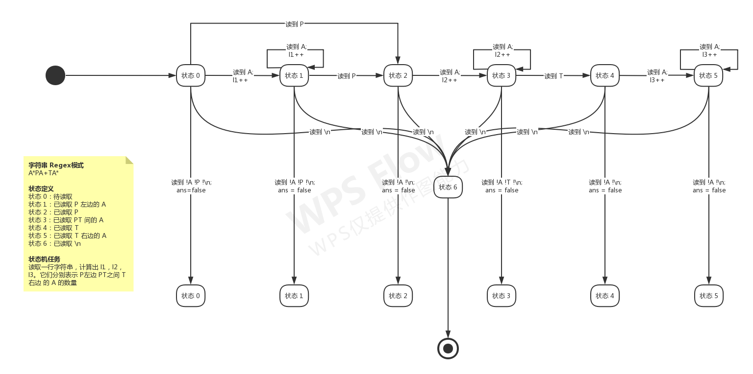
有限状态机 Finite State Machine

针对字符串处理的相关题目,可以使用 FSM 解决。首先分清楚两个概念

  • 有限的状态节点
  • 表示状态转移条件的有向边

在做题时,首先定义好要解决问题的字符串模式,接下来定义有穷的状态码及其内涵,最后找到所有的可状态转移条件。

例子

PAT B1003 “我要通过”,点此处,并在以下目录 solutions/solutions-PAT/B1003.cpp 中查看题解。其 FSM 图如下: B1003 FSM

PAT A1060 “Are They Equal”,点此处,并在以下目录 solutions/solutions-PAT/A1060.cpp 中查看题解。

KMP 算法 Knuth–Morris–Pratt string-searching algorithm

代码模板
 1
 2
 3
 4
 5
 6
 7
 8
 9
10
11
12
13
14
15
16
17
18
19
20
21
22
23
24
25
26
27
28
29
30
31
32
33
34
35
36
37
38
39
40
41
42
43
44
45
46
47
48
49
50
51
52
53
54
55
56
// 代码参考王道教程

#include <iostream>
#include <cstring>
#define MAXN 50
using namespace std;
char s[MAXN], t[MAXN];
int ls, lt, nxt[MAXN] = {0};

void get_next()
{
    int i = 1, j = 0;
    nxt[1] = 0;
    while (i <= ls)
    {
        if (j == 0 || s[i] == t[j])
        {
            i++; j++;

            // 初级的方法
            // nxt[i] = j;

            // 高级的方法
            if (s[i] != s[j]) nxt[i] = j;
            else nxt[i] = nxt[j];
        }
        else
            j = nxt[j];
    }
}

int kmp_index()
{
    int i = 1, j = 1;
    while (i <= ls && j <= lt)
    {
        if (j == 0 || s[i] == t[j])
        {
            i++;
            j++;
        }
        else
            j = nxt[j];
    }
    if (j > lt) return i - lt;
    else return 0;
}

int main()
{
    cin >> s+1 >> t+1;
    ls = strlen(s+1);
    lt = strlen(t+1);
    cout << kmp_index();
    return 0;
}

Citation

@article{shichaosong2021cc,
  title = {C/C++ 语言算法与数据结构学习笔记},
  author = {Shichao Song},
  journal = {The Kiseki Log},
  year = {2021},
  month = {February},
  url = {https://ki-seki.github.io/posts/210205-algorithm/}
}

References


  1. 胡凡, and 曾磊. 算法笔记. 机械工业出版社, July 2026. ↩︎