)](https://ki-seki.github.io/posts/261025-training-data-retrieval/assets/semantic-islands-cover.png)
Introduction
Training a large text-to-image model from scratch calls for an interactive image–text retrieval and cluster-browsing tool built over the full training data. It lets research and data teams find and inspect data at the level of both samples and clusters, and look at each sample’s content, annotations and source. Its three main uses are:
- Filtering, cleaning and mixing pretraining data. Browse clusters and their representative samples to check the data distribution; review and remove NSFW or otherwise unqualified samples and clusters under established safety and quality policies; and adjust the sampling weights and quotas of clusters or data sources (for example, upsampling high-quality landscapes and designs) to raise or lower their share of the training set.
- Recovering and selecting post-training data. Around a model’s weak spots, target examples and specific capability needs, retrieve and recover candidate samples from the data pool, then turn them into datasets through human selection, quality checks and annotation where needed. These datasets support targeted capability gains in SFT and RL, such as text rendering, detailed portraits or particular styles.
- Checking for evaluation data leakage. Use evaluation images, or the reference images behind evaluation prompts, as queries, one at a time or in batches, to find identical and near-duplicate training samples and check whether training and evaluation data overlap.
Building a retrieval system at this scale is far from trivial. In this post, I’ll use a retrieval system with 1.4 billion image–text samples as an example, and I’ll walk through its design and implementation.
Related Work
Searching billion-scale image–text training data. The closest public system is LAION’s clip-retrieval, built for the LAION-5B dataset1. Beaumont2 describes computing CLIP embeddings for its five billion images on 32 A100 GPUs, compressing them into an 800 GB product-quantized index with autofaiss, and serving it from a single machine through memory mapping. Vespa’s billion-scale vector search series3 uses the same data to study serving architectures built on an HNSW-indexed inverted file. These systems offer general search over an open dataset, whereas ours serves in-house training data.
Vector compression and search. Beyond the original papers on product quantization4 and FAISS5, Pinecone’s guide to product quantization6 and McCormick’s IVF-PQ tutorial7 are gentler introductions to the mechanisms shown in Figures 4–6 below.
Embedding-based data curation. Clustering in embedding space is also widely used to curate pretraining data. Vo et al.8 apply hierarchical k-means and balanced sampling to build curated datasets automatically, SemDeDup9 removes semantic near-duplicates within k-means clusters, and NVIDIA NeMo Curator10 packages CLIP embedding, quality filtering and semantic deduplication into a GPU pipeline. The cluster browser and mixing tool described later serve a similar purpose but keep people in the loop. For exploring embeddings interactively, Nomic Atlas11 offers a similar 2D map with vector search.
Existing write-ups tend to cover one piece: how an open dataset was indexed, how product quantization works, or how to curate data by clustering. This post puts the whole path in one place, from how the data is stored, through embedding extraction and building and querying an IVF-PQ index, to the tools a data team uses day to day. Each step is grounded in a real deployment over 1.4B samples, with measured throughput, the actual index specifications and the engineering choices behind them.
Data Storage Format and Management
First, the storage format. Logically, the data is one huge table keyed by image. Each image’s most important sidecar is its text caption; we are training a text-to-image model, after all. Other sidecars may include layout, tags, source, aesthetic scores and various category labels.
Physically, we store the image data on its own as sharded main parquets12, which hold the image bytes or references to them. All other associated information lives in sidecar parquets that are row-aligned with the main parquets, which keeps images and their attributes efficient to manage and access. Every sample is located by the triple (dataset_revision_id, source_file_id, source_row), that is, the dataset revision, the source shard and the row within that shard, which gives uniform access and traceability back to the source.
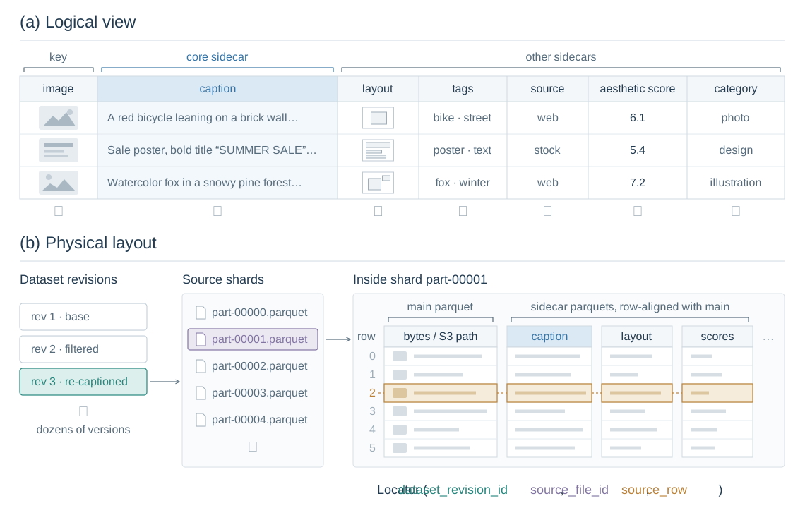
Figure 1: Logical view and physical layout of the data. A sample is located by the triple of dataset revision, source shard and row within the shard.
This way of managing data serves the needs of both the data team and the training team:
- What the data team needs. Filtering, resampling and re-annotation over large-scale, multi-stage training can produce dozens of derived datasets or versions, which makes the data harder to manage and samples harder to trace.
- What the training team needs. As little data-processing overhead as possible during training: quickly locating the needed samples with simple predicate filters, and avoiding repeated reads and decodes of image data, so training runs efficiently. However, the data inside a shard can also be unevenly distributed, so the data team may need to resample or adjust it within a shard to keep the training data balanced.
Offline Index Construction
At billions of samples, exact search is out of the question, so the system has to be a nearest-neighbor search system. In short: compute embeddings that map samples into a vector space, then retrieve with a nearest-neighbor algorithm, in our case IVF-PQ4 from FAISS513.
The build consists mainly of organizing the input manifest and sample mapping, extracting image embeddings, clustering and vector quantization, building the sharded index, and integrity checks, as shown in Figure 2.
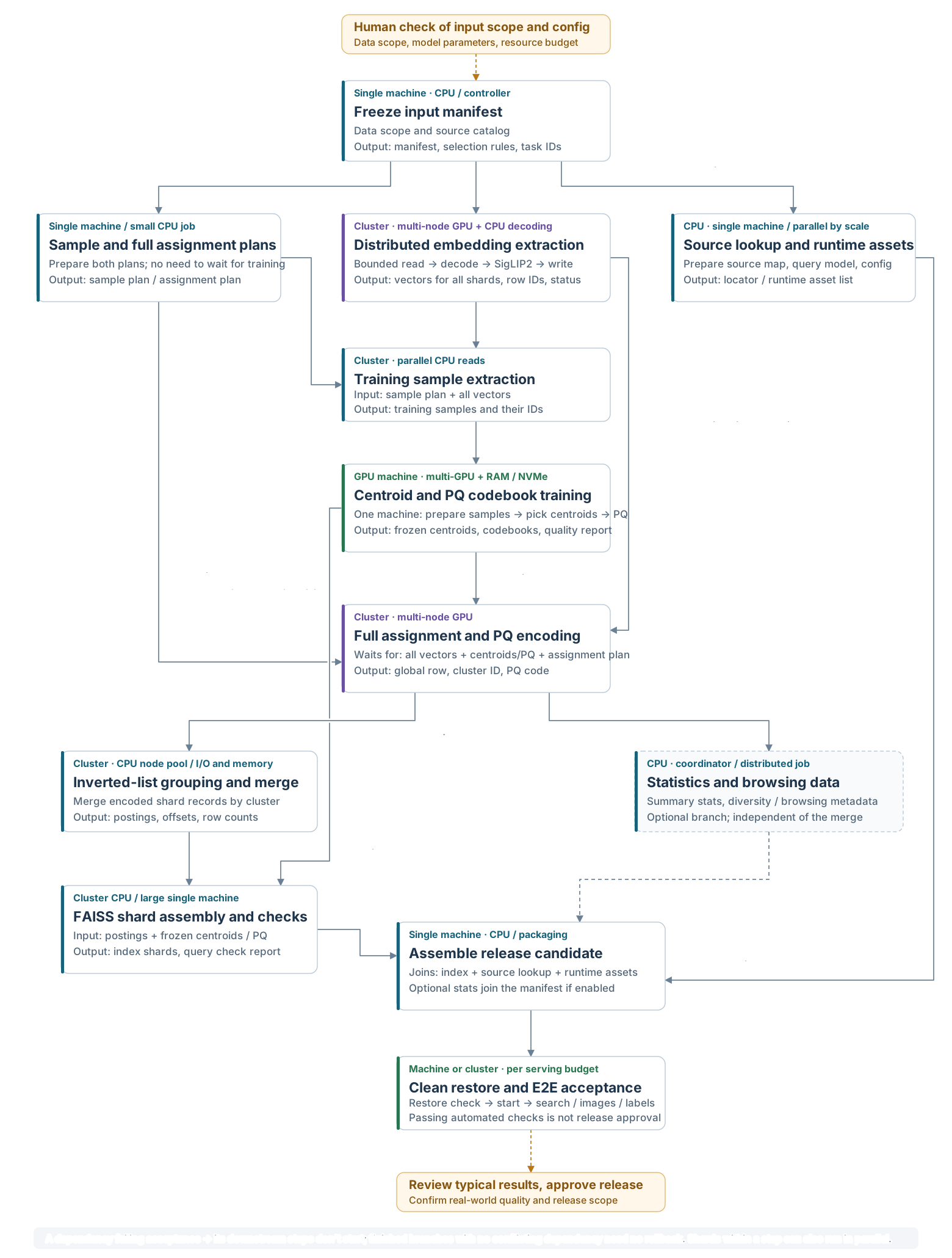
Figure 2: Stage dependencies and resource allocation of the offline index build. Solid lines are required artifact dependencies, grey dashed lines are optional capability dependencies, and orange dashed lines are human sign-offs; actual concurrency depends on the resource budget and orchestration policy.
A retrieval system over text-to-image training data usually has to support both text and image semantic queries, so text and images must map into the same vector space. That generally calls for a model trained with image–text contrastive learning1415; here we use SigLIP216 to extract image embeddings. On top of FAISS, we then combine an inverted file index (IVF)17 with product quantization (PQ)4 to build a compressed retrieval index, which keeps search efficient while cutting storage substantially. The following sections cover distributed embedding extraction, clustering and compressed indexing, and building the full index.
Distributed Embedding Extraction
Embedding extraction is the most compute-intensive step of the build: it has to schedule work efficiently across a cluster, overlap data preparation with inference, and keep the GPUs busy.
Inputs and Model
We organize the input manifest according to the data in scope for retrieval, with Parquet shards as the processing unit, recording each source file’s location and row count. Images can be read either from the image bytes embedded in a shard or from the S3 path recorded in it, and are then decoded, resized and pixel-normalized with a fixed configuration.
Images are encoded with SigLIP2 SO400M (patch14, 384 × 384 input), which produces a 1,152-dimensional vector for each valid image; the vectors are L2-normalized and stored in FP16. Online queries use the image or text encoder of the same model, mapping reference images and text into a shared embedding space, so a single image index supports both image-to-image and text-to-image search.
Scaling Out
For billions of images, embedding extraction involves not only GPU inference but also object-storage reads, image decoding and writing results. Each Parquet shard is one task: we estimate the initial load from shard sizes, assign tasks to multiple compute nodes, and process them in parallel with several GPU worker processes per node, each shard writing its results independently.
Different image formats and sizes, and varying storage read latency, make task durations uneven. We improve throughput on three fronts, task scheduling, data feeding and inference batching:
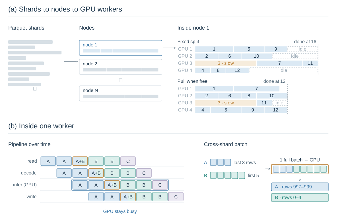
Figure 3: Distributed embedding extraction. (a) Shards are assigned to nodes by estimated load, and GPU workers within a node claim the next shard whenever they are free, which avoids the long tail a slow shard causes under a fixed split. (b) Within one worker, reading, decoding, inference and writing overlap, and ready images from different shards can fill one batch, with results written back by original shard and row. Durations and row numbers are illustrative.
- Dynamic task scheduling within a node. A worker that finishes a task goes on to claim the next unprocessed shard, with a small claim-ahead window. This keeps a few workers from piling up slow tasks while others sit idle, eases load imbalance and the long tail at the end of a run, and shortens the time to finish the whole batch.
- Pipeline overlap and bounded prefetch. While the GPU computes the current batch, later data is prepared in advance so that reading, decoding and inference overlap as much as possible and the GPU spends less time waiting for data. The number of shards in flight per worker is capped to avoid over-using resources.
- Cross-shard batching. Within one worker, ready images from different Parquet shards that share a decode path are merged into one inference batch. This reduces small batches caused by shard boundaries or data filtering and raises batch fill. Results are still written back by original shard and row, so every vector stays matched to its sample.
These choices came from what we saw in production, where extraction was largely I/O-bound. A typical Parquet shard was 300–500 MiB and downloaded at a median of 26–28 MiB/s, so while SigLIP2 needed only 3–5 seconds for a 1,000-image shard, the slowest downloads took 20–75 seconds. With the optimizations above in place, we measured end-to-end throughput on a single node with eight NVIDIA RTX PRO 6000 GPUs:
| Images | Per node | Per GPU |
|---|---|---|
| Web photos, mostly JPEG | ~1,750 images/s | ~220 images/s |
| Large design images, ≥ 2048 px | ~530 images/s | ~66 images/s |
Shards dominated by large PNGs are the slow tail, at about 12 images/s per GPU, which is why the dynamic scheduling above matters.
Implementation
In code, I’d avoid Ray actors or any other distributed processing framework. Plain Python is enough: an SPMD design with one process per GPU launched by torchrun, a node-local queue from which processes claim shards, and asynchronous I/O. That schedules work efficiently and correctly.
Checkpointing and Validation
Lastly, to reduce recomputation after a long job is interrupted, we checkpoint by data block within each shard. After the build, we check the coverage and row counts of source shards against the outputs, summarize download, decode and other failures, and spot-check the sample-ID mapping as well as the dimension, data type and L2 norm of the vectors. Failed samples keep their original position and status, so that dropping records outright never shifts row numbers; missing or abnormal outputs are fixed and reviewed before delivery.
Clustering and Compressed Indexing
At one 1,152-dimensional FP16 vector per image, a billion images take 2.304 TB for the vector values alone (decimal units, excluding images, annotations and file-format overhead). That is too much memory to serve, and comparing against every vector is far too slow for real-time search. We use IVF-PQ, which combines narrowing the search scope with vector compression.
IVF Clustering
IVF needs clustering to obtain its centroids, and PQ codebook training also clusters each subspace separately, after the IVF centroids are fixed (see below), so both start with a clustering step. Clustering over the full data is very slow, so we usually train on a smaller sample of N vectors.
As an example, take the reference build configuration of the 1.4B pretraining library, with N = 100M vectors. Quotas are allocated in proportion to the row counts of the input embedding shards, then each shard is sampled by stratified row ranges and read by row range. This stratified block sampling takes advantage of ranged reads from object storage, avoiding downloading a whole vector file just to take a few samples; it is not independent, row-by-row, globally uniform random sampling. The sample is split into 99 million IVF training vectors and 1 million held-out vectors, which are used only to evaluate clustering at this stage.
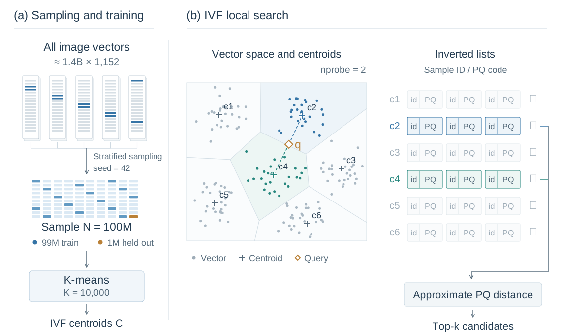
Figure 4: IVF sampling, centroid training and search scope, using the reference build configuration of the 1.4B pretraining library as an example. The 2D cluster positions and probed region are illustrative.
The number of IVF clusters is set to K=10,000, and training learns the centroid positions from the 99 million vectors above. All vectors are then assigned to their nearest centroid, and the samples of each cluster are organized into an inverted list. At query time, the system first finds the centroids closest to the query vector and then scans only their lists, avoiding a pass over the whole dataset.
PQ Compression and Encoding
For compression, we apply product quantization (PQ) to the residual, the difference between a vector and its assigned centroid. We resample from the same 100M-vector sample (again to speed up clustering, so not all 100M vectors are used), allocating read quotas evenly across sample shards. This yields 2.1 million vectors: 2 million for PQ training and 0.1 million held out to evaluate quantization reconstruction error.
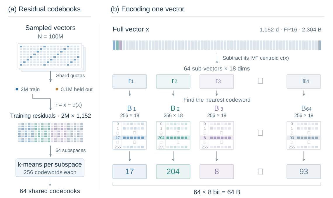
Figure 5: Sampled codebook training and full encoding for PQ64. The codebooks are shared across the whole index.
The number of PQ segments and bits per segment are also set by configuration. Here we use PQ64 with 64 segments of 8 bits each: each segment has 18 dimensions, and its 8-bit code indexes one of 256 codewords in that segment’s sub-codebook. We first compute the residuals of the PQ training samples against the already fixed IVF centroids, then gather the sub-vectors at the same segment position across all IVF clusters and run 256-way k-means on each, giving 64 codebooks shared across the whole index.
To encode, each residual sub-vector picks the nearest codeword in its codebook and stores only that codeword’s ID, from 0 to 255. A 1,152-dimensional FP16 vector that took 2,304 bytes is thus represented by a 64-byte quantized code.
How an IVF-PQ Query Works
In the finished IVF-PQ index, each entry of an inverted list stores only a sample ID and a 64-byte PQ code, not the original vector. Queries never decode codes back into vectors either: approximate distances come straight from table lookups, in four steps, as shown in Figure 6.
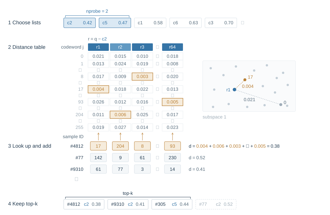
Figure 6: Computing approximate distances in an IVF-PQ query. Values and sample IDs are illustrative.
- Choose inverted lists. Compute the distance from the query vector q to all 10,000 centroids and search only the inverted lists of the nearest
nprobeclusters, skipping the rest. - Build a distance table. PQ encodes a vector’s residual relative to its centroid, so for each probed list we first compute the query residual r = q − c and cut it into 64 segments of 18 dimensions, the same way as in encoding. We then compute the distance from each segment to the 256 codewords of its sub-codebook, giving a 64 × 256 distance table. It is computed once per list and shared by every entry in that list.
- Look up and add. Each of an entry’s 64 codes picks one cell in its segment’s column of the distance table; adding up those 64 values gives the approximate distance between q and that sample. Each entry costs only 64 lookups and additions, with no vector decoding, which is why PQ can scan large numbers of candidates quickly.
- Keep the nearest k. Pool the entries from all probed lists and keep the k with the smallest approximate distances as candidates.
Building the Full Index
Once the centroids and PQ codebooks are fixed, assigning all vectors to clusters and encoding them can run in a distributed way. Sample IDs and quantized codes are then merged by cluster and assembled into several FAISS index shards, so that no single index file is too large to load and query efficiently; all shards of an index share the same centroids and codebooks. The number of clusters, the PQ code length and the number of clusters probed at query time (nprobe) together determine resource cost and retrieval quality: probing more clusters usually improves recall but scans more candidates, while PQ trades quantization error for lower storage and scan cost, so recall from this index is approximate.
Taking the 1.4B-sample library as an example, the resulting index has the following specifications:
| Samples | 1,386,418,079, from 1,264 embedding shards |
| Embeddings | SigLIP2 SO400M, 1,152-d FP16; about 3.19 TB of raw vectors |
| Distance | Squared L2 on normalized vectors, equivalent to cosine similarity |
| IVF | K = 10,000, spherical mini-batch k-means1819; 99 million training and 1 million held-out vectors; after full assignment all 10,000 lists are non-empty, with 297–946,850 entries per list |
| PQ | 64 segments × 8 bits, 18 dimensions and 256 codewords per segment; 2 million training and 0.1 million held-out vectors; 64 bytes per vector |
| Index shards | 8, split by contiguous cluster ID, about 1,250 clusters and 167–180 million entries each; 12.1–13.0 GB per shard, 100.2 GB in total, about 1/32 of the raw vectors |
| Build | Full assignment and encoding in 64 parallel tasks; about 1.6–3.6 minutes to assemble each shard; each shard read back and checked with nprobe = 32; about 7.3 hours from finishing the 100M sample to passing the checks |
| Serving | One shard per GPU across 8 GPUs; default nprobe = 32, so each query scans only 0.32% of the lists, about 4.4 million codes at the average list length |
Online Retrieval System
Image–Text Semantic Search Service
Online retrieval accepts reference images, text, or both. The system generates a normalized query vector with the same SigLIP2 encoder used to build the index. Multiple images, or images plus text, can either be pooled into a single query vector first, or retrieved separately and fused by similarity or rank20. Each query route searches all index shards in parallel, and the server merges and deduplicates results by sample ID and keeps candidates sorted by approximate PQ distance.

Figure 7: How one online query is processed.
Result browsing ties the retrieval ranking to each sample’s content, annotations and source. From a thumbnail, users can open the details to see the caption, the raw JSON, a display image aligned with the annotations, and the dataset revision, source file path and row number, as shown in Figure 8.

Figure 8: An example of the search interface.
Cluster Browsing and Data Mixing
Cleaning and mixing pretraining data happens mostly at the cluster level. We provide a browsing tool organized around the clusters from offline clustering: each cluster carries automatically generated, searchable semantic labels and can be sorted by aesthetics, tightness or diversity; samples within a cluster are ordered by cosine similarity to the cluster center, so the content and quality of a cluster can be judged at a glance. The cluster centers are projected to 2D with UMAP21 and can be browsed interactively to see the overall data distribution.
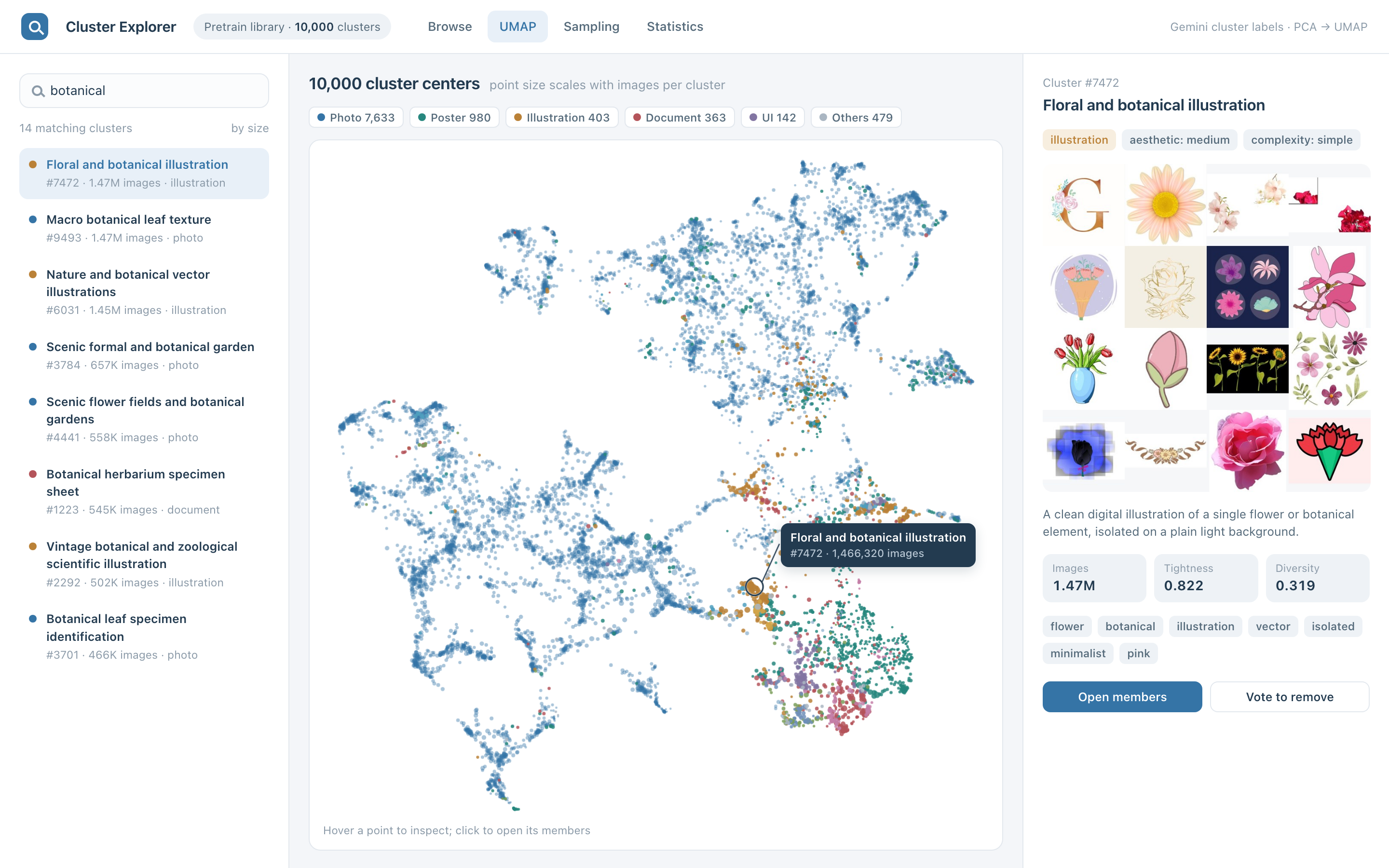
Figure 9: An example of the cluster-browsing interface.
On top of this, several annotators can vote on low-quality or non-compliant clusters and export a removal list, and a mixing tool solves for sampling quotas over clusters × datasets: once researchers set target shares for each data source, the tool exports the corresponding sampling plan.
Other Features
AI-assisted programming made it easy for the system to offer extra features. These are the ones we use most in practice:
- Batch independent queries. For a set of model failure cases or evaluation samples, batch queries run each one separately so results can be compared side by side, instead of submitting single queries over and over. Researchers can narrow candidates by attributes such as data source and size, gather hand-picked samples into collections that persist across queries, and export a JSONL list with source paths and row numbers for downstream data recovery, review and re-annotation. Query parameters and result snapshots can also be saved as share links, so a team can review the same set of candidates together.
- Result verification. For a chosen number of top candidates, the system reads the source images back, regenerates full vectors with the current encoding configuration, computes cosine similarity without PQ approximation, and can rerank within those candidates. It also computes pHash22 Hamming distances and compares file SHA-256 hashes, flagging near-duplicates and byte-identical images.
- More flexible query combinations. Multiple reference images can be combined in three ways: common features (averaging the vectors), any reference (searching each separately and taking the best), and consensus (rank fusion, which resists being pulled off course by one outlier image). When both images and text are given, a slider sets their relative weight, 80% image and 20% text by default. Any result can be used as a new query or added as a reference with one click, and a storage path can be pasted directly as a query image.
- And more.
Conclusion
This post described methods for retrieving and managing large-scale image training data, covering data storage and management, embedding construction, clustering and compressed indexing, and the workflows and technical details of online retrieval and sample inspection.
Citation
@article{elliotsong2026abillionscalere,
  title = {A Billion-Scale Retrieval System for Text-to-Image Training Data},
  author = {Elliot Song},
  journal = {The Kiseki Log},
  year = {2026},
  month = {October},
  url = {https://ki-seki.github.io/posts/261025-training-data-retrieval/}
}
References
-
Schuhmann, Christoph, et al. “LAION-5B: An Open Large-Scale Dataset for Training Next Generation Image-Text Models.” Advances in Neural Information Processing Systems 35 (Datasets and Benchmarks Track), 2022. arXiv, https://arxiv.org/abs/2210.08402. ↩︎
-
Beaumont, Romain. “Semantic Search at Billions Scale.” Medium, 31 Mar. 2022, https://rom1504.medium.com/semantic-search-at-billions-scale-95f21695689a. ↩︎
-
Bergum, Jo Kristian. “Building Billion-Scale Vector Search: Part Two.” Vespa Blog, 26 Oct. 2022, https://blog.vespa.ai/building-billion-scale-vector-search-part-two/. ↩︎
-
Jégou, Hervé, Matthijs Douze, and Cordelia Schmid. “Product Quantization for Nearest Neighbor Search.” IEEE Transactions on Pattern Analysis and Machine Intelligence, vol. 33, no. 1, 2011, pp. 117–128. IEEE Xplore, https://doi.org/10.1109/TPAMI.2010.57. ↩︎ ↩︎ ↩︎
-
Douze, Matthijs, et al. The Faiss Library. 2024. arXiv, https://arxiv.org/abs/2401.08281. ↩︎ ↩︎
-
Pinecone. “Product Quantization: Compressing High-Dimensional Vectors by 97%.” Faiss: The Missing Manual, https://www.pinecone.io/learn/series/faiss/product-quantization/. ↩︎
-
McCormick, Chris. “Product Quantizers for k-NN Tutorial Part 2.” 22 Oct. 2017, https://mccormickml.com/2017/10/22/product-quantizer-tutorial-part-2/. ↩︎
-
Vo, Huy V., et al. “Automatic Data Curation for Self-Supervised Learning: A Clustering-Based Approach.” Transactions on Machine Learning Research, 2024. arXiv, https://arxiv.org/abs/2405.15613. ↩︎
-
Abbas, Amro, et al. SemDeDup: Data-Efficient Learning at Web-Scale through Semantic Deduplication. 2023. arXiv, https://arxiv.org/abs/2303.09540. ↩︎
-
NVIDIA. “About Image Curation.” NeMo Curator Documentation, https://docs.nvidia.com/nemo/curator/latest/curate-images/index.html. ↩︎
-
Nomic AI. “Nomic Atlas.” https://atlas.nomic.ai/. ↩︎
-
The Apache Software Foundation. “Apache Parquet.” https://parquet.apache.org/. ↩︎
-
Johnson, Jeff, Matthijs Douze, and Hervé Jégou. “Billion-Scale Similarity Search with GPUs.” IEEE Transactions on Big Data, vol. 7, no. 3, 2021, pp. 535–547. arXiv, https://arxiv.org/abs/1702.08734. ↩︎
-
Radford, Alec, et al. “Learning Transferable Visual Models From Natural Language Supervision.” Proceedings of the 38th International Conference on Machine Learning, vol. 139, Proceedings of Machine Learning Research, 2021, pp. 8748–8763. PMLR, https://proceedings.mlr.press/v139/radford21a.html. ↩︎
-
Zhai, Xiaohua, et al. “Sigmoid Loss for Language Image Pre-Training.” Proceedings of the IEEE/CVF International Conference on Computer Vision, 2023, pp. 11975–11986. arXiv, https://arxiv.org/abs/2303.15343. ↩︎
-
Tschannen, Michael, et al. SigLIP 2: Multilingual Vision-Language Encoders with Improved Semantic Understanding, Localization, and Dense Features. 20 Feb. 2025. arXiv, https://arxiv.org/abs/2502.14786. ↩︎
-
Sivic, Josef, and Andrew Zisserman. “Video Google: A Text Retrieval Approach to Object Matching in Videos.” Proceedings of the Ninth IEEE International Conference on Computer Vision, 2003. IEEE Xplore, https://doi.org/10.1109/ICCV.2003.1238663. ↩︎
-
Dhillon, Inderjit S., and Dharmendra S. Modha. “Concept Decompositions for Large Sparse Text Data Using Clustering.” Machine Learning, vol. 42, 2001, pp. 143–175. Springer, https://doi.org/10.1023/A:1007612920971. ↩︎
-
Sculley, D. “Web-Scale K-Means Clustering.” Proceedings of the 19th International Conference on World Wide Web, ACM, 2010, pp. 1177–1178. ACM Digital Library, https://doi.org/10.1145/1772690.1772862. ↩︎
-
Cormack, Gordon V., Charles L. A. Clarke, and Stefan Büttcher. “Reciprocal Rank Fusion Outperforms Condorcet and Individual Rank Learning Methods.” Proceedings of the 32nd International ACM SIGIR Conference on Research and Development in Information Retrieval, ACM, 2009, pp. 758–759. ACM Digital Library, https://doi.org/10.1145/1571941.1572114. ↩︎
-
McInnes, Leland, John Healy, and James Melville. UMAP: Uniform Manifold Approximation and Projection for Dimension Reduction. 2018. arXiv, https://arxiv.org/abs/1802.03426. ↩︎
-
Zauner, Christoph. Implementation and Benchmarking of Perceptual Image Hash Functions. Master’s thesis, Upper Austria University of Applied Sciences, 2010. https://www.phash.org/docs/pubs/thesis_zauner.pdf. ↩︎