)](https://ki-seki.github.io/posts/260531-lilian-rl-overview/RL_illustration_new.png)
This is a fully annotated guide to Lilian Weng’s post A (Long) Peek into Reinforcement Learning. I also added an extra section, Key Formulas at a Glance, to summarize the key formulas in the post for quick reference.
I recommend reading the Multi-armed Bandit post first if you are new to RL.
What is Reinforcement Learning?
Say, we have an agent in an unknown environment and this agent can obtain some rewards by interacting with the environment. The agent ought to take actions so as to maximize cumulative rewards. In reality, the scenario could be a bot playing a game to achieve high scores, or a robot trying to complete physical tasks with physical items; and not just limited to these.
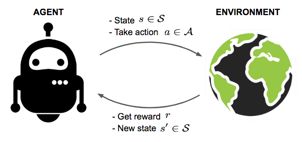
An agent interacts with the environment, trying to take smart actions to maximize cumulative rewards.
The goal of Reinforcement Learning (RL) is to learn a good strategy for the agent from experimental trials and relative simple feedback received. With the optimal strategy, the agent is capable to actively adapt to the environment to maximize future rewards.
Key Concepts
Now Let’s formally define a set of key concepts in RL.
The agent is acting in an environment. How the environment reacts to certain actions is defined by a model which we may or may not know. The agent can stay in one of many states ($s \in \mathcal{S}$) of the environment, and choose to take one of many actions ($a \in \mathcal{A}$) to switch from one state to another. Which state the agent will arrive in is decided by transition probabilities between states ($P$). Once an action is taken, the environment delivers a reward ($r \in \mathcal{R}$) as feedback.
The model defines the reward function and transition probabilities. We may or may not know how the model works and this differentiate two circumstances:
- Know the model: planning with perfect information; do model-based RL. When we fully know the environment, we can find the optimal solution by Dynamic Programming (DP). Do you still remember “longest increasing subsequence” or “traveling salesmen problem” from your Algorithms 101 class? LOL. This is not the focus of this post though.
- Does not know the model: learning with incomplete information; do model-free RL or try to learn the model explicitly as part of the algorithm. Most of the following content serves the scenarios when the model is unknown.
More about model-based content:
We say model-based RL when the transition probabilities are knowable or we can write down the Bellman equations. Let’s use LIS (Longest Increasing Subsequence) as an example.
Bellman equation for the value function is:
$$ V(s) = \max_a \sum_{s'} P(s'|s,a)[R + \gamma V(s')] $$In LIS, the transition probability is deterministic, meaning that if we take action a in state s, we will always arrive at the same state s’ and get the same reward R. Thus
$$ P(s'|s,a) = 1. $$And the reward is also deterministic,
$$ R(s, a) = 1. $$As for the gamma, we can set it to be 1 because we do not need to discount future rewards in this case.
$$ \gamma = 1. $$So,
$$ V(s) = \max_a [1 + V(s')] $$This is exactly the same as the DP solution for LIS:
$$ dp[i] = 1 + \max_{j < i,\, a[j] < a[i]} dp[j] $$The agent’s policy $\pi(s)$ provides the guideline on what is the optimal action to take in a certain state with the goal to maximize the total rewards. Each state is associated with a value function $V(s)$ predicting the expected amount of future rewards we are able to receive in this state by acting the corresponding policy. In other words, the value function quantifies how good a state is. Both policy and value functions are what we try to learn in reinforcement learning.
.)](/posts/260531-lilian-rl-overview/RL_algorithm_categorization.png)
Summary of approaches in RL based on whether we want to model the value, policy, or the environment. (Image source: reproduced from David Silver’s RL course lecture 1.)
The interaction between the agent and the environment involves a sequence of actions and observed rewards in time, $t=1, 2, \dots, T$. During the process, the agent accumulates the knowledge about the environment, learns the optimal policy, and makes decisions on which action to take next so as to efficiently learn the best policy. Let’s label the state, action, and reward at time step t as $S_t$, $A_t$, and $R_t$, respectively. Thus the interaction sequence is fully described by one episode (also known as “trial” or “trajectory”) and the sequence ends at the terminal state $S_T$:
$$ S_1, A_1, R_2, S_2, A_2, \dots, S_T $$In multi-armed bandit problems, there is no state transition, so the episode is simply:
$$S, A, R, S_T \; \text{with } S=S_T$$And the learning process is across multiple episodes.
Why is the index of reward $t+1$?
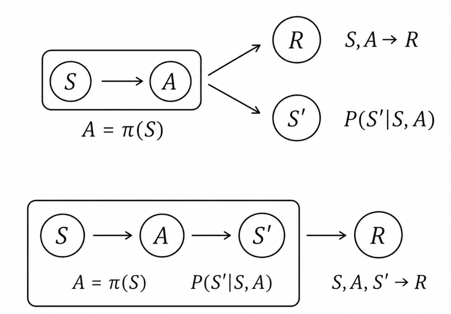
Two common types of dependency structures in MDP episodes.
Terms you will encounter a lot when diving into different categories of RL algorithms:
- Model-based: Rely on the model of the environment; either the model is known or the algorithm learns it explicitly.
- Model-free: No dependency on the model during learning.
- On-policy: Use the deterministic outcomes or samples from the target policy to train the algorithm.
- Off-policy: Training on a distribution of transitions or episodes produced by a different behavior policy rather than that produced by the target policy.
Model: Transition and Reward
The model is a descriptor of the environment. With the model, we can learn or infer how the environment would interact with and provide feedback to the agent. The model has two major parts, transition probability function $P$ and reward function $R$.
Let’s say when we are in state s, we decide to take action a to arrive in the next state s’ and obtain reward r. This is known as one transition step, represented by a tuple (s, a, s’, r).
The transition function P records the probability of transitioning from state s to s’ after taking action a while obtaining reward r. We use $\mathbb{P}$ as a symbol of “probability”.
$$ P(s', r \vert s, a) = \mathbb{P} [S_{t+1} = s', R_{t+1} = r \vert S_t = s, A_t = a] $$Thus the state-transition function can be defined as a function of $P(s', r \vert s, a)$:
$$ P_{ss'}^a = P(s' \vert s, a) = \mathbb{P} [S_{t+1} = s' \vert S_t = s, A_t = a] = \sum_{r \in \mathcal{R}} P(s', r \vert s, a) $$The reward function R predicts the next reward triggered by one action:
$$ R(s, a) = \mathbb{E} [R_{t+1} \vert S_t = s, A_t = a] = \sum_{r\in\mathcal{R}} r \sum_{s' \in \mathcal{S}} P(s', r \vert s, a) $$If you’re familiar with Multi-armed Bernoulli Bandit problems (Learn it here), you may understand formulas above as a generalization of the bandit setting.
Bandit problem is stateless, so
$$ P_{ss'}^a = P(s' \vert s, a) = 1 $$And the reward function is simply the expected reward of taking action a:
$$ R(s, a) = \sum_{r\in\mathcal{R}} r \sum_{s' \in \{s'\}} P(s', r \vert s, a) = \sum_{r\in\mathcal{R}} r P(r \vert s, a) \\= 1 \cdot P(r=1 \vert s, a) + 0 \cdot P(r=0 \vert s, a) = \theta_a $$Here is one thing we should pay attention to, the difference between reward function and expected reward function.
There’s no fixed convention on their notations, so I list some possible notations for both of them in the table below:
| Immediate Reward | Expected Reward | |
|---|---|---|
| Scenario 1 | $R(s, a, s')$ | $R(s, a)$ |
| Scenario 2 | $r$ | $\mathbb{E}[r]$ |
Policy
Policy, as the agent’s behavior function $\pi$, tells us which action to take in state s. It is a mapping from state s to action a and can be either deterministic or stochastic:
- Deterministic: $\pi(s) = a$.
- Stochastic: $\pi(a \vert s) = \mathbb{P}_\pi [A=a \vert S=s]$.
The relation between deterministic and stochastic policy:
$$ \pi(a\mid s) = \begin{cases} 1 & a = \pi(s) \\ 0 & a \neq \pi(s) \end{cases} $$Value Function
Value function measures the goodness of a state or how rewarding a state or an action is by a prediction of future reward. The future reward, also known as return, is a total sum of discounted rewards going forward. Let’s compute the return $G_t$ starting from time t:
$$ G_t = R_{t+1} + \gamma R_{t+2} + \dots = \sum_{k=0}^{\infty} \gamma^k R_{t+k+1} $$The discounting factor $\gamma \in [0, 1]$ penalize the rewards in the future, because:
- The future rewards may have higher uncertainty; i.e. stock market.
- The future rewards do not provide immediate benefits; i.e. As human beings, we might prefer to have fun today rather than 5 years later ;).
- Discounting provides mathematical convenience; i.e., we don’t need to track future steps forever to compute return.
- We don’t need to worry about the infinite loops in the state transition graph.
Let’s furthermore clarify the last two points.
- If we do not discount the future rewards, then the return is simply the sum of all future rewards. Then it will never converge. But with discounting factor $\gamma < 1$, the return is a geometric series and it converges to a finite value.
- If there is no discount factor, the agent will decide that staying in that loop forever is the “optimal” strategy because the total reward will eventually reach infinity.
Proof of convergence of return with discounting factor:
Assume there exists some positive finite constant $R_{\max}$ such that $|R_t| \le R_{\max}$ for all $t$.
Then we have:
$$ \begin{aligned} |G_t| &= |R_{t+1} + \gamma R_{t+2} + \dots| \\ &\leq |R_{t+1}| + |\gamma R_{t+2}| + \dots & \text{ ; triangle inequality } \\ &\leq |R_{\max}| + |\gamma R_{\max}| + \dots \\ &\leq R_{\max} + \gamma R_{\max} + \dots \\ &= R_{\max} \sum_{k=0}^{\infty} \gamma^k \\ &= \frac{R_{\max}}{1 - \gamma} & \text{ ; infinite geometric series } \\ &< \infty \end{aligned} $$The state-value of a state s is the expected return if we are in this state at time t, $S_t = s$:
$$ V_{\pi}(s) = \mathbb{E}_{\pi}[G_t \vert S_t = s] $$Similarly, we define the action-value (“Q-value”; Q as “Quality” I believe?) of a state-action pair as:
$$ Q_{\pi}(s, a) = \mathbb{E}_{\pi}[G_t \vert S_t = s, A_t = a] $$Additionally, since we follow the target policy $\pi$, we can make use of the probability distribution over possible actions and the Q-values to recover the state-value:
$$ V_{\pi}(s) = \sum_{a \in \mathcal{A}} Q_{\pi}(s, a) \pi(a \vert s) $$The difference between action-value and state-value is the action advantage function (“A-value”):
$$ A_{\pi}(s, a) = Q_{\pi}(s, a) - V_{\pi}(s) $$Summary so far:
- Policy weights your choices.
- Transition Probability weights the environment’s outcomes.
- Value Functions are the result of averaging these weighted rewards over time.
The relation between immediate reward, return, and value functions:
- Immediate reward: at state s, take action a, get reward r.
- Return: the total discounted reward starting from state s and action a, following policy $\pi$.
- Value functions: other forms of return, but with different conditions. State-value function is the expected return given state s, while action-value function is the expected return given state s and action a.
Let’s use GRPO as the example to rewrite some functions above.
GRPO is stateless, so we have:
$$ \begin{aligned} G_t &= R_{t+1} \text{ ; since there is no state transition} \\ Q_{\pi}(a) &= \mathbb{E}_{\pi}[G_t \vert A_t = a] \approx r_a \\ V_{\pi}(s) &= \mathbb{E}_{\pi}[G_t \vert S_t = s] = \sum_{a \in \mathcal{A}} Q_{\pi}(a) \pi(a \vert s) = \sum_{a \in \mathcal{A}} r_a \frac{1}{|\mathcal{A}|} = \bar{r} \\ A_{\pi}(s, a) &= Q_{\pi}(s, a) - V_{\pi}(s) = r_a - \bar{r} \end{aligned} $$This is very close to the real GRPO advantage function:
.)](/posts/260531-lilian-rl-overview/GRPO_Advantage.png)
GRPO Advantage Function (Image source: DeepSeekMath: Pushing the Limits of Mathematical Reasoning in Open Language Models.)
Except that the real GRPO advantage is z-score normalized.
Optimal Value and Policy
The optimal value function produces the maximum return:
$$ V_{*}(s) = \max_{\pi} V_{\pi}(s), Q_{*}(s, a) = \max_{\pi} Q_{\pi}(s, a) $$The optimal policy achieves optimal value functions:
$$ \pi_{*} = \arg\max_{\pi} V_{\pi}(s), \pi_{*} = \arg\max_{\pi} Q_{\pi}(s, a) $$And of course, we have $V_{\pi_{*}}(s)=V_{*}(s)$ and $Q_{\pi_{*}}(s, a) = Q_{*}(s, a)$.
Best policy → best value functions → best return.
Markov Decision Processes
In more formal terms, almost all the RL problems can be framed as Markov Decision Processes (MDPs). All states in MDP has “Markov” property, referring to the fact that the future only depends on the current state, not the history:
$$ \mathbb{P}[ S_{t+1} \vert S_t ] = \mathbb{P} [S_{t+1} \vert S_1, \dots, S_t] $$Or in other words, the future and the past are conditionally independent given the present, as the current state encapsulates all the statistics we need to decide the future.
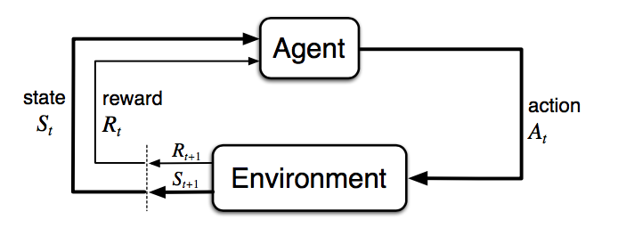
The agent-environment interaction in a Markov decision process. (Image source: Sec. 3.1 Sutton & Barto (2017).)
A Markov deicison process consists of five elements $\mathcal{M} = \langle \mathcal{S}, \mathcal{A}, P, R, \gamma \rangle$, where the symbols carry the same meanings as key concepts in the previous section, well aligned with RL problem settings:
- $\mathcal{S}$ - a set of states;
- $\mathcal{A}$ - a set of actions;
- $P$ - transition probability function;
- $R$ - reward function;
- $\gamma$ - discounting factor for future rewards. In an unknown environment, we do not have perfect knowledge about $P$ and $R$.
)](/posts/260531-lilian-rl-overview/mdp_example.jpg)
A fun example of Markov decision process: a typical work day. (Image source: randomant.net/reinforcement-learning-concepts)
Bellman Equations
Bellman equations refer to a set of equations that decompose the value function into the immediate reward plus the discounted future values.
$$ \begin{aligned} V(s) &= \mathbb{E}[G_t \vert S_t = s] \\ &= \mathbb{E} [R_{t+1} + \gamma R_{t+2} + \gamma^2 R_{t+3} + \dots \vert S_t = s] \\ &= \mathbb{E} [R_{t+1} + \gamma (R_{t+2} + \gamma R_{t+3} + \dots) \vert S_t = s] \\ &= \mathbb{E} [R_{t+1} + \gamma G_{t+1} \vert S_t = s] \\ &= \mathbb{E} [R_{t+1} + \gamma V(S_{t+1}) \vert S_t = s] \end{aligned} $$Similarly for Q-value,
$$ \begin{aligned} Q(s, a) &= \mathbb{E} [R_{t+1} + \gamma V(S_{t+1}) \mid S_t = s, A_t = a] \\ &= \mathbb{E} [R_{t+1} + \gamma \mathbb{E}_{a\sim\pi} Q(S_{t+1}, a) \mid S_t = s, A_t = a] \end{aligned} $$Bear in mind that:
- state value function is
- the weighted average of action value function
- over the action distribution defined by the policy $\pi$
Bellman Expectation Equations
The recursive update process can be further decomposed to be equations built on both state-value and action-value functions. As we go further in future action steps, we extend V and Q alternatively by following the policy $\pi$.
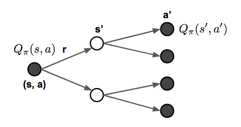
Illustration of how Bellman expection equations update state-value and action-value functions.
Bellman Optimality Equations
If we are only interested in the optimal values, rather than computing the expectation following a policy, we could jump right into the maximum returns during the alternative updates without using a policy. RECAP: the optimal values $V_*$ and $Q_*$ are the best returns we can obtain, defined in the section on optimal value and policy.
$$ \begin{aligned} V_*(s) &= \max_{a \in \mathcal{A}} Q_*(s,a)\\ Q_*(s, a) &= R(s, a) + \gamma \sum_{s' \in \mathcal{S}} P_{ss'}^a V_*(s') \\ V_*(s) &= \max_{a \in \mathcal{A}} \big( R(s, a) + \gamma \sum_{s' \in \mathcal{S}} P_{ss'}^a V_*(s') \big) \\ Q_*(s, a) &= R(s, a) + \gamma \sum_{s' \in \mathcal{S}} P_{ss'}^a \max_{a' \in \mathcal{A}} Q_*(s', a') \end{aligned} $$Unsurprisingly they look very similar to Bellman expectation equations.
If we have complete information of the environment, this turns into a planning problem, solvable by DP. Unfortunately, in most scenarios, we do not know $P_{ss'}^a$ or $R(s, a)$, so we cannot solve MDPs by directly applying Bellmen equations, but it lays the theoretical foundation for many RL algorithms.
The key equation is the Bellman optimality equation for Q-value:
$$ Q_*(s, a) = R(s, a) + \gamma \sum_{s' \in \mathcal{S}} P_{ss'}^a \max_{a' \in \mathcal{A}} Q_*(s', a') $$Because it connects the environment (transition probability and reward), the optimal action-value function and the optimal action selection process.
Why is the Bellman optimality equation for Q-value the way it is? Let’s derive it step by step.
Firstly, if we select the optimal action with 100% probability, then the state-value function is the same as the action-value function:
$$V_{*}(s) = \max_{a \in \mathcal{A}} Q_*(s, a)$$Let’s recall the Q-value decomposition in Bellman Expectation Equations:
$$Q(s, a) = R(s, a) + \gamma \sum_{s' \in \mathcal{S}} P_{ss'}^a V (s')$$So we have:
$$Q_*(s, a) = R(s, a) + \gamma \sum_{s' \in \mathcal{S}} P_{ss'}^a V_* (s')$$Then we can substitute $V_*(s')$ with $\max_{a' \in \mathcal{A}} Q_*(s', a')$:
$$\boxed{Q_*(s, a) = R(s, a) + \gamma \sum_{s' \in \mathcal{S}} P_{ss'}^a \max_{a' \in \mathcal{A}} Q_*(s', a')}$$Common Approaches
Dynamic Programming
When the model is fully known, following Bellman equations, we can use Dynamic Programming (DP) to iteratively evaluate value functions and improve policy.
Policy Evaluation
Policy Evaluation is to compute the state-value $V_\pi$ for a given policy $\pi$:
$$ V_{t+1}(s) = \mathbb{E}_\pi [r + \gamma V_t(s') | S_t = s] = \sum_a \pi(a \vert s) \sum_{s', r} P(s', r \vert s, a) (r + \gamma V_t(s')) $$Policy Improvement
Based on the value functions, Policy Improvement generates a better policy $\pi' \geq \pi$ by acting greedily.
$$ Q_\pi(s, a) = \mathbb{E} [R_{t+1} + \gamma V_\pi(S_{t+1}) \vert S_t=s, A_t=a] = \sum_{s', r} P(s', r \vert s, a) (r + \gamma V_\pi(s')) $$Policy Iteration
The Generalized Policy Iteration (GPI) algorithm refers to an iterative procedure to improve the policy when combining policy evaluation and improvement.
$$ \pi_0 \xrightarrow[]{\text{evaluation}} V_{\pi_0} \xrightarrow[]{\text{improve}} \pi_1 \xrightarrow[]{\text{evaluation}} V_{\pi_1} \xrightarrow[]{\text{improve}} \pi_2 \xrightarrow[]{\text{evaluation}} \dots \xrightarrow[]{\text{improve}} \pi_* \xrightarrow[]{\text{evaluation}} V_* $$In GPI, the value function is approximated repeatedly to be closer to the true value of the current policy and in the meantime, the policy is improved repeatedly to approach optimality. This policy iteration process works and always converges to the optimality, but why this is the case?
Say, we have a policy $\pi$ and then generate an improved version $\pi'$ by greedily taking actions, $\pi'(s) = \arg\max_{a \in \mathcal{A}} Q_\pi(s, a)$. The value of this improved $\pi'$ is guaranteed to be better because:
$$ \begin{aligned} Q_\pi(s, \pi'(s)) &= Q_\pi(s, \arg\max_{a \in \mathcal{A}} Q_\pi(s, a)) \\ &= \max_{a \in \mathcal{A}} Q_\pi(s, a) \geq Q_\pi(s, \pi(s)) = V_\pi(s) \end{aligned} $$- Policy evaluation:
- $V_{t+1}(s) = \sum_a \pi(a \vert s) \sum_{s', r} P(s', r \vert s, a) (r + \gamma V_t(s'))$
- $Q_\pi(s, a) = \sum_{s', r} P(s', r \vert s, a) (r + \gamma V_\pi(s'))$
- Policy improvement:
- $\pi'(s) = \arg\max_{a \in \mathcal{A}} Q_\pi(s, a)$
- Policy iteration:
- $\pi_0 \xrightarrow[]{\text{evaluation}} V_{\pi_0} \xrightarrow[]{\text{improve}}\pi_1$
Derivation of policy evaluation mainly decomposes it into the $\langle \mathcal{S}, \mathcal{A}, P, R, \gamma \rangle$ components.
For state-value:
$$ \begin{align} V_{t+1}(s) &= \mathbb{E}_\pi \big[ r + \gamma V_t(s') \,\big|\, S_t = s \big] &\text{ , by definition of } V_\pi \\ &= \sum_a \pi(a|s) \, \mathbb{E}\big[ r + \gamma V_t(s') \,\big|\, s, a \big] & \text{ , expectation over actions} \\ &= \sum_a \pi(a|s) \sum_{s',r} P(s',r \mid s,a) \, \big[ r + \gamma V_t(s') \big] & \text{ , expectation over } s, a \rightarrow s', r \\ \end{align} $$For action-value:
$$ \begin{align} Q_\pi(s, a) &= \mathbb{E} [R_{t+1} + \gamma V_\pi(S_{t+1}) \vert S_t=s, A_t=a] \\ &= \sum_{s', r} P(s', r \vert s, a) (r + \gamma V_\pi(s')) \end{align} $$Pseudo code of policy iteration:
$$ \begin{array}{l} \textbf{Algorithm: Policy Iteration} \\ \textbf{Input: } \text{State space } \mathcal{S}, \text{ Action space } \mathcal{A}, \\ \quad \text{Transition probabilities } P(s', r \mid s,a) \\ \quad \text{Reward function } r=R(s,a,s'), \\ \quad \text{Discount factor } \gamma, \\ \quad \text{Initial policy } \pi_0 \\ \textbf{Output: } \text{Optimal policy } \pi^*, \text{ Optimal value function } V^* \\ \pi \leftarrow \pi_0 \\ \textbf{Repeat:} \\ \quad \text{Policy Evaluation:} \\ \quad \quad V(s) \leftarrow \sum_a \pi(a|s) \sum_{s', r} P(s', r|s,a)\,[r + \gamma V(s')] \\ \quad \quad Q(s, a) \leftarrow \sum_{s', r} P(s', r|s,a)\,[r + \gamma V(s')] \\ \quad \text{Policy Improvement:} \\ \quad \quad \pi'(s) \leftarrow \arg\max_{a \in \mathcal{A}} Q_\pi(s, a) \\ \quad \text{If } \pi' = \pi \\ \quad \text{Or } \|V_{t+1} - V_t\| < \epsilon \text{ (value function converged)} \\ \quad \text{Or iteration count } > N_{\max} \text{ (iteration limit)} \\ \quad \quad \text{Then stop and return } (\pi, V) \\ \quad \text{Else } \pi \leftarrow \pi' \\ \textbf{Until convergence} \end{array} $$Relation between $P(s'|s,a)$, $P(s', r|s,a)$, and $R(s,a,s')$:
$$ P(s'|s,a) = \sum_{r \in \mathcal{R}} P(s', r|s,a) $$Monte-Carlo Methods
First, let’s recall that $V(s) = \mathbb{E}[ G_t \vert S_t=s]$. Monte-Carlo (MC) methods uses a simple idea: It learns from episodes of raw experience without modeling the environmental dynamics and computes the observed mean return as an approximation of the expected return. To compute the empirical return $G_t$, MC methods need to learn from complete episodes $S_1, A_1, R_2, \dots, S_T$ to compute $G_t = \sum_{k=0}^{T-t-1} \gamma^k R_{t+k+1}$ and all the episodes must eventually terminate.
The empirical mean return for state s is:
$$ V(s) = \frac{\sum_{t=1}^T \mathbb{1}[S_t = s] G_t}{\sum_{t=1}^T \mathbb{1}[S_t = s]} $$where $\mathbb{1}[S_t = s]$ is a binary indicator function. We may count the visit of state $s$ every time so that there could exist multiple visits of one state in one episode (“every-visit”), or only count it the first time we encounter a state in one episode (“first-visit”). This way of approximation can be easily extended to action-value functions by counting (s, a) pair.
$$ Q(s, a) = \frac{\sum_{t=1}^T \mathbb{1}[S_t = s, A_t = a] G_t}{\sum_{t=1}^T \mathbb{1}[S_t = s, A_t = a]} $$To learn the optimal policy by MC, we iterate it by following a similar idea to GPI.
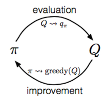
Monte Carlo control algorithm
- Improve the policy greedily with respect to the current value function: $\pi(s) = \arg\max_{a \in \mathcal{A}} Q(s, a)$.
- Generate a new episode with the new policy $\pi$ (i.e. using algorithms like $\epsilon$-greedy helps us balance between exploitation and exploration.)
- Estimate Q using the new episode: $Q_\pi(s, a) = \frac{\sum_{t=1}^T \big( \mathbb{1}[S_t = s, A_t = a] \sum_{k=0}^{T-t-1} \gamma^k R_{t+k+1} \big)}{\sum_{t=1}^T \mathbb{1}[S_t = s, A_t = a]}$
Monte Carlo is a model-free method, we no longer need the transition probabilities $P(s', r \mid s,a)$ or the reward function $R(s,a,s')$ as inputs. Instead, we rely on generating complete episodes to calculate the empirical returns.
$$\begin{array}{l} \textbf{Algorithm: Monte Carlo Control} \\ \textbf{Input: } \text{State space } \mathcal{S}, \text{ Action space } \mathcal{A}, \\ \quad \text{Discount factor } \gamma, \\ \quad \text{Exploration parameter } \epsilon \\ \textbf{Output: } \text{Optimal policy } \pi^*, \text{ Optimal action-value function } Q^* \\ \text{Initialize } Q(s,a) \text{ arbitrarily for all } s \in \mathcal{S}, a \in \mathcal{A} \\ \pi \leftarrow \text{initial } \epsilon\text{-greedy policy} \\ \textbf{Repeat:} \\ \quad \text{Episode Generation:} \\ \quad \quad \text{Generate a complete episode } S_1, A_1, R_2, \dots, S_T \text{ following } \pi \\ \quad \text{Policy Evaluation:} \\ \quad \quad \text{For each } (s,a) \text{ in the episode:} \\ \quad \quad \quad Q_\pi(s, a) \leftarrow \frac{\sum_{t=1}^T \big( \mathbb{1}[S_t = s, A_t = a] \sum_{k=0}^{T-t-1} \gamma^k R_{t+k+1} \big)}{\sum_{t=1}^T \mathbb{1}[S_t = s, A_t = a]} \\ \quad \text{Policy Improvement:} \\ \quad \quad \pi'(s) \leftarrow \arg\max_{a \in \mathcal{A}} Q_\pi(s, a) \text{ (Greedy improvement)} \\ \quad \quad \pi \leftarrow \epsilon\text{-greedy}(\pi') \text{ (Balance exploitation and exploration)} \\ \quad \text{If } \|Q_{i+1} - Q_i\| < \delta \text{ (action-value function converged)} \\ \quad \text{Or episode count } > N_{\max} \text{ (iteration limit)} \\ \quad \quad \text{Then stop and return } (\pi, Q) \\ \textbf{Until convergence} \end{array}$$Temporal-Difference Learning
Bootstrapping
The name comes from the phrase:
“Pull yourself up by your own bootstraps.”
Meaning:
You improve your estimate using your own previous estimate.
Value Estimation
The key idea in TD learning is to update the value function $V(S_t)$ towards an estimated return $R_{t+1} + \gamma V(S_{t+1})$ (known as “TD target”). To what extent we want to update the value function is controlled by the learning rate hyperparameter $\alpha$:
$$ \begin{aligned} V(S_t) &\leftarrow (1- \alpha) V(S_t) + \alpha G_t \\ V(S_t) &\leftarrow V(S_t) + \alpha (G_t - V(S_t)) \\ V(S_t) &\leftarrow V(S_t) + \alpha (R_{t+1} + \gamma V(S_{t+1}) - V(S_t)) \end{aligned} $$Similarly, for action-value estimation:
$$Q(S_t, A_t) \leftarrow Q(S_t, A_t) + \alpha (R_{t+1} + \gamma Q(S_{t+1}, A_{t+1}) - Q(S_t, A_t))$$Next, let’s dig into the fun part on how to learn optimal policy in TD learning (aka “TD control”). Be prepared, you are gonna see many famous names of classic algorithms in this section.
MC state value estimation:
$$V(s) = \frac{\sum_{t=1}^T \mathbb{1}[S_t = s] G_t}{\sum_{t=1}^T \mathbb{1}[S_t = s]}$$MC target:
$$G_t = \underbrace{R_{t+1} + \gamma R_{t+2} + \gamma^2 R_{t+3} + \dots}_{\text{Real rewards from episode}}$$TD target:
$$G_t \approx \underbrace{R_{t+1}}_{\text{Real reward}} + \underbrace{\gamma V(S_{t+1})}_{\text{Estimated part}}$$When we say “target” in RL, we mean:
This is the future return we want to know. But the true return is unknown (and may never be fully observed), we must estimate it—using either full returns (MC) or bootstrapped estimates (TD).
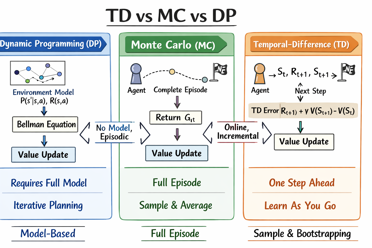
Comparison between TD, MC and DP.
SARSA: On-Policy TD control
“SARSA” refers to the procedure of updaing Q-value by following a sequence of …, $S_t$, $A_t$, $R_{t+1}$, $S_{t+1}$, $A_{t+1}$, …. The idea follows the same route of GPI. Within one episode, it works as follows:
- Initialize $t = 0$.
- Start with $S_0$ and choose action $A_0 = \arg\max_{a \in \mathcal{A}} Q(S_0, a)$, where $\epsilon$-greedy is commonly applied.
- At time $t$, after applying action $A_t$, we observe reward $R_{t+1}$ and get into the next state $S_{t+1}$.
- Then pick the next action in the same way as in step 2: $A_{t+1} = \arg\max_{a \in \mathcal{A}} Q(S_{t+1}, a)$.
- Update the Q-value function: $Q(S_t, A_t) \leftarrow Q(S_t, A_t) + \alpha (R_{t+1} + \gamma Q(S_{t+1}, A_{t+1}) - Q(S_t, A_t))$.
- Set $t = t + 1$ and repeat from step 3.
In each step of SARSA, we need to choose the next action according to the current policy.
In SARSA, behavior policy (sampling action) = target policy (learning Q values):
$$ \pi(a|s)=\epsilon\frac{1}{|\mathcal{A}|} + (1-\epsilon)\,\mathbf{1}[a=\arg\max_{a'}Q(s,a')] $$Q-Learning: Off-policy TD control
The development of Q-learning (Watkins & Dayan, 1992) is a big breakout in the early days of Reinforcement Learning. Within one episode, it works as follows:
- Initialize $t = 0$.
- Starts with $S_0$.
- At time step $t$, we pick the action according to Q values, $A_t = \arg\max_{a \in \mathcal{A}} Q(S_t, a)$ and $\epsilon$-greedy is commonly applied.
- After applying action $A_t$, we observe reward $R_{t+1}$ and get into the next state $S_{t+1}$.
- Update the Q-value function: $Q(S_t, A_t) \leftarrow Q(S_t, A_t) + \alpha (R_{t+1} + \gamma \max_{a \in \mathcal{A}} Q(S_{t+1}, a) - Q(S_t, A_t))$.
- $t = t + 1$ and repeat from step 3.
The key difference from SARSA is that Q-learning does not follow the current policy to pick the second action $A_{t+1}$. It estimates $Q^*$ out of the best Q values, but which action (denoted as $a^*$) leads to this maximal Q does not matter and in the next step Q-learning may not follow $a^*$.
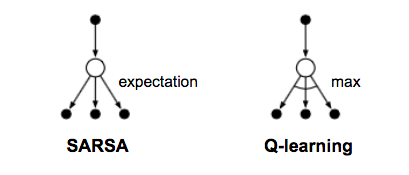
SARSA vs Q-learning comparison
P.S. Red part is the TD target.
Q-learning behavior policy ($\epsilon$-greedy):
$$ \mu(a|s)=\frac{\epsilon}{|\mathcal{A}|} + (1-\epsilon)\,\mathbf{1}[a=\arg\max_{a'}Q(s,a')] $$Q-learning target policy (greedy):
$$ \pi(a|s)=\mathbf{1}[a=\arg\max_{a'}Q(s,a')] $$Deep Q-Network
Theoretically, we can memorize $Q^*(.)$ for all state-action pairs in Q-learning, like in a gigantic table. However, it quickly becomes computationally infeasible when the state and action space are large. Thus people use functions (i.e. a machine learning model) to approximate Q values and this is called function approximation. For example, if we use a function with parameter $\theta$ to calculate Q values, we can label Q value function as $Q(s, a; \theta)$.
Unfortunately Q-learning may suffer from instability and divergence when combined with a nonlinear Q-value function approximation and bootstrapping (See Problems #2).
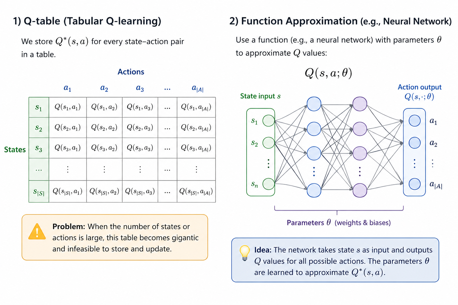
Q-Table vs Q-Network
Deep Q-Network (“DQN”; Mnih et al. 2015) aims to greatly improve and stabilize the training procedure of Q-learning by two innovative mechanisms:
Experience Replay: All the episode steps $e_t = (S_t, A_t, R_t, S_{t+1})$ are stored in one replay memory $D_t = \{ e_1, \dots, e_t \}$. $D_t$ has experience tuples over many episodes. During Q-learning updates, samples are drawn at random from the replay memory and thus one sample could be used multiple times. Experience replay improves data efficiency, removes correlations in the observation sequences, and smooths over changes in the data distribution. Periodically Updated Target: Q is optimized towards target values that are only periodically updated. The Q network is cloned and kept frozen as the optimization target every $C$ steps ($C$ is a hyperparameter). This modification makes the training more stable as it overcomes the short-term oscillations.
The loss function looks like this:
$$\mathcal{L}(\theta) = \mathbb{E}_{(s, a, r, s') \sim U(D)} \Big[ \big( r + \gamma \max_{a'} Q(s', a'; \theta^{-}) - Q(s, a; \theta) \big)^2 \Big]$$where $U(D)$ is a uniform distribution over the replay memory $D$; $\theta^{-}$ is the parameters of the frozen target Q-network.
In addition, it is also found to be helpful to clip the error term to be between [-1, 1]. (I always get mixed feeling with parameter clipping, as many studies have shown that it works empirically but it makes the math much less pretty. :/)
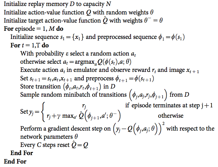
Deep Q-Network algorithm
There are many extensions of DQN to improve the original design, such as DQN with dueling architecture (Wang et al. 2016) which estimates state-value function $V(s)$ and advantage function $A(s, a)$ with shared network parameters.
Combining TD and MC Learning
In the previous section on value estimation in TD learning, we only trace one step further down the action chain when calculating the TD target. One can easily extend it to take multiple steps to estimate the return.
Let’s label the estimated return following $n$ steps as $G_t^{(n)}$, $n = 1, \dots, \infty$, then:
| $n$ | $G_t^{(n)}$ | Notes |
|---|---|---|
| $n = 1$ | $G_t^{(1)} = R_{t+1} + \gamma V(S_{t+1})$ | TD learning |
| $n = 2$ | $G_t^{(2)} = R_{t+1} + \gamma R_{t+2} + \gamma^2 V(S_{t+2})$ | |
| $\dots$ | ||
| $n = n$ | $G_t^{(n)} = R_{t+1} + \gamma R_{t+2} + \dots + \gamma^{n-1} R_{t+n} + \gamma^n V(S_{t+n})$ | |
| $\dots$ | ||
| $n = \infty$ | $G_t^{(\infty)} = R_{t+1} + \gamma R_{t+2} + \dots + \gamma^{T-t-1} R_T + \gamma^{T-t} V(S_T)$ | MC estimation |
The generalized n-step TD learning still has the same form for updating the value function:
$$V(S_t) \leftarrow V(S_t) + \alpha (G_t^{(n)} - V(S_t))$$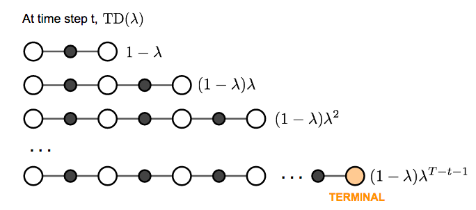
TD($\lambda$) eligibility traces diagram
We are free to pick any $n$ in TD learning as we like. Now the question becomes what is the best $n$? Which $G_t^{(n)}$ gives us the best return approximation? A common yet smart solution is to apply a weighted sum of all possible n-step TD targets rather than to pick a single best $n$. The weights decay by a factor $\lambda$ with $n$, $\lambda^{n-1}$; the intuition is similar to why we want to discount future rewards when computing the return: the more future we look into the less confident we would be. To make all the weight ($n \rightarrow \infty$) sum up to 1, we multiply every weight by $(1-\lambda)$, because:
$$ \begin{aligned} \text{let } S &= 1 + \lambda + \lambda^2 + \dots \\ S &= 1 + \lambda(1 + \lambda + \lambda^2 + \dots) \\ S &= 1 + \lambda S \\ S &= 1 / (1-\lambda) \end{aligned} $$This weighted sum of many n-step returns is called $\lambda$-return $G_t^{\lambda} = (1-\lambda) \sum_{n=1}^{\infty} \lambda^{n-1} G_t^{(n)}$. TD learning that adopts $\lambda$-return for value updating is labeled as TD($\lambda$). The original version we introduced above is equivalent to TD(0).
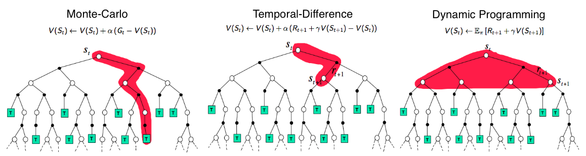
Comparison of TD, MC, and DP backup diagrams
Here are the algorithmic details of TD($\lambda$). But we don’t explain why here.
TD($\lambda$) update (backward view) This is the actual algorithm:
Eligibility trace:
\[ e_t(s)=\gamma\lambda e_{t-1}(s)+\mathbf{1}[S_t=s] \]TD error:
\[ \delta_t = R_{t+1} + \gamma V(S_{t+1}) - V(S_t) \]Value update:
\[ V(s) \leftarrow V(s) + \alpha\,\delta_t\, e_t(s) \]Why backward view = forward view (equivalence)
\[ G_t^\lambda - V(S_t) = \sum_{k=t}^{\infty} (\gamma\lambda)^{k-t}\,\delta_k \]Meaning:
- Forward view λ‑return = weighted mixture of all n‑step returns
- Backward view = weighted mixture of all future TD errors
- Weights are identical → \((\gamma\lambda)^{k-t}\)
So:
Forward view defines what TD(λ) should learn. Backward view implements the same weights efficiently.
Policy Gradient
- Value-based RL: learn the value function $V$ or $Q$, and select actions indirectly through them.
- Policy Gradient RL: directly learn a parameterized policy $\pi(a \mid s; \theta)$ with the objective of maximizing the expected return.
In discrete space:
$$\mathcal{J}(\theta) = V_{\pi_\theta}(S_1) = \mathbb{E}_{\pi_\theta}[V_1]$$where $S_1$ is the initial starting state.
Or in continuous space:
$$\mathcal{J}(\theta) = \sum_{s \in \mathcal{S}} d_{\pi_\theta}(s) V_{\pi_\theta}(s) = \sum_{s \in \mathcal{S}} \Big( d_{\pi_\theta}(s) \sum_{a \in \mathcal{A}} \pi(a|s, \theta) Q_\pi(s, a) \Big)$$where $d_{\pi_\theta}(s)$ is stationary distribution of Markov chain for $\pi_\theta$. If you are unfamiliar with the definition of a “stationary distribution,” please check this reference.
Errata 1:
Here, the equality $V_{\pi_\theta}(S_1) = \mathbb{E}_{\pi_\theta}[V_1]$ is not strictly rigorous and should be viewed as a slight abuse of notation.
We only need to understand that we aim to maximize $\mathcal{J}(\theta)$, which is the expected return starting from the initial state $S_1$.
Errata 2:
The second formula is also in discrete space.
Stationary distribution $d_{\pi_\theta}(s)$ is the probability of $s$ when the Markov chain system evolves for a long time and converges.
Example: 7‑DoF Robotic Arm
Action:
\[ a \in \mathbb{R}^7 \](continuous joint velocities/torques).
Value‑based RL (Q‑learning / DQN)
- Must learn \(Q(s,a)\) where \(a\) is a 7‑dim continuous vector.
- Requires \(\arg\max_a Q(s,a)\) → impossible (high‑dim non‑convex optimization).
- Q‑network input is huge → unstable.
- No natural exploration in continuous actions.
→ Not practical for robotic arms.
Policy‑based RL (Policy Gradient / PPO / SAC)
- Learn \(\pi(a|s)\) directly.
- Network outputs Gaussian parameters: \[ \mu_\theta(s),\ \sigma_\theta(s) \in \mathbb{R}^7 \]
- Action sampled as: \[ a = \mu_\theta(s) + \sigma_\theta(s)\epsilon \]
- No argmax needed; exploration comes from \(\sigma\).
- Stable and standard for continuous control.
→ The dominant approach for robotic manipulators.
Policy Gradient Theorem
Computing the gradient numerically can be done by perturbing $\theta$ by a small amount $\epsilon$ in the k-th dimension. It works even when $\mathcal{J}(\theta)$ is not differentiable (nice!), but unsurprisingly very slow.
$$ \frac{\partial \mathcal{J}(\theta)}{\partial \theta_k} \approx \frac{\mathcal{J}(\theta + \epsilon u_k) - \mathcal{J}(\theta)}{\epsilon} $$Or analytically,
$$\mathcal{J}(\theta) = \mathbb{E}_{\pi_\theta}[r] = \sum_{s \in \mathcal{S}} d_{\pi_\theta}(s) \sum_{a \in \mathcal{A}} \pi(a|s; \theta) R(s, a)$$Because it is impossible for us to get the gradient of $d_{\pi_\theta}$, we have to use the perturbation-based estimation trick.
Actually we have nice theoretical support for (replacing $d(.)$ with $d_\pi(.)$):
$$\mathcal{J}(\theta) = \sum_{s \in \mathcal{S}} d_{\pi_\theta}(s) \sum_{a \in \mathcal{A}} \pi(a|s; \theta) Q_\pi(s, a) \propto \sum_{s \in \mathcal{S}} d(s) \sum_{a \in \mathcal{A}} \pi(a|s; \theta) Q_\pi(s, a)$$Check Sec 13.1 in Sutton & Barto (2017) for why this is the case.
Then,
$$ \begin{aligned} \mathcal{J}(\theta) &= \sum_{s \in \mathcal{S}} d(s) \sum_{a \in \mathcal{A}} \pi(a \vert s; \theta) Q_\pi(s, a) \\ \nabla \mathcal{J}(\theta) &= \sum_{s \in \mathcal{S}} d(s) \sum_{a \in \mathcal{A}} \nabla \pi(a \vert s; \theta) Q_\pi(s, a) \\ &= \sum_{s \in \mathcal{S}} d(s) \sum_{a \in \mathcal{A}} \pi(a \vert s; \theta) \frac{\nabla \pi(a \vert s; \theta)}{\pi(a \vert s; \theta)} Q_\pi(s, a) \\ &= \sum_{s \in \mathcal{S}} d(s) \sum_{a \in \mathcal{A}} \pi(a \vert s; \theta) \nabla \ln \pi(a \vert s; \theta) Q_\pi(s, a) \\ &= \mathbb{E}_{\pi_\theta} [\nabla \ln \pi(a \vert s; \theta) Q_\pi(s, a)] \end{aligned} $$This result is named “Policy Gradient Theorem” which lays the theoretical foundation for various policy gradient algorithms:
$$\nabla \mathcal{J}(\theta) = \mathbb{E}_{\pi_\theta}[\nabla \ln \pi(a|s, \theta) Q_\pi(s, a)]$$The core is we can get rid of the $\theta$-parameterized stationary distribution and then we can use sampling to get input-output pairs to get gradients.
REINFORCE
REINFORCE, also known as Monte-Carlo policy gradient, relies on $Q_\pi(s, a)$, an estimated return by MC methods using episode samples, to update the policy parameter $\theta$.
A commonly used variation of REINFORCE is to subtract a baseline value from the return $G_t$ to reduce the variance of gradient estimation while keeping the bias unchanged. For example, a common baseline is state-value, and if applied, we would use $A(s, a) = Q(s, a) - V(s)$ in the gradient ascent update.
- Initialize $\theta$ at random
- Generate one episode $S_1, A_1, R_2, S_2, A_2, \dots, S_T$
- For $t=1, 2, \dots, T$:
- Estimate the the return $G_t$ since the time step $t$.
- $\theta \leftarrow \theta + \alpha \gamma^t G_t \nabla \ln \pi(A_t|S_t, \theta)$.
Actor-Critic
If the value function is learned in addition to the policy, we would get Actor-Critic algorithm.
- Critic: updates value function parameters $w$ and depending on the algorithm it could be action-value $Q(a|s; w)$ or state-value $V(s; w)$.
- Actor: updates policy parameters $\theta$, in the direction suggested by the critic, $\pi(a|s; \theta)$.
Let’s see how it works in an action-value actor-critic algorithm.
- Initialize $s, \theta, w$ at random; sample $a \sim \pi(a|s; \theta)$.
- For $t = 1 \dots T$:
- Sample reward $r_t \sim R(s, a)$ and next state $s' \sim P(s'|s, a)$.
- Then sample the next action $a' \sim \pi(a'|s'; \theta)$.
- Update policy parameters: $\theta \leftarrow \theta + \alpha_\theta Q(s, a; w) \nabla_\theta \ln \pi(a|s; \theta)$.
- Compute the correction for action-value at time $t$: $G_{t:t+1} = r_t + \gamma Q(s', a'; w) - Q(s, a; w)$ and use it to update value function parameters: $w \leftarrow w + \alpha_w G_{t:t+1} \nabla_w Q(s, a; w)$.
- Update $a \leftarrow a'$ and $s \leftarrow s'$.
$\alpha_\theta$ and $\alpha_w$ are two learning rates for policy and value function parameter updates, respectively.
In essence, this is the combination of DQN and REINFORCE.
A3C
Asynchronous Advantage Actor-Critic (Mnih et al., 2016), short for A3C, is a classic policy gradient method with the special focus on parallel training.
In A3C, the critics learn the state-value function, $V(s; w)$, while multiple actors are trained in parallel and get synced with global parameters from time to time. Hence, A3C is good for parallel training by default, i.e. on one machine with multi-core CPU.
The loss function for state-value is to minimize the mean squared error, $\mathcal{J}_v(w) = (G_t - V(s; w))^2$ and we use gradient descent to find the optimal $w$. This state-value function is used as the baseline in the policy gradient update.
Here is the algorithm outline:
We have global parameters, $\theta$ and $w$; similar thread-specific parameters, $\theta'$ and $w'$. Initialize the time step $t = 1$ While $T \leq T_{MAX}$:
-
Reset gradient: $d\theta = 0$ and $dw = 0$.
-
Synchronize thread-specific parameters with global ones: $\theta' = \theta$ and $w' = w$.
-
$t_{start} = t$ and get $s_t$.
-
While ($s_t \neq$ TERMINAL) and ($t - t_{start} \leq t_{max}$):
- Pick the action $a_t \sim \pi(a_t|s_t; \theta')$ and receive a new reward $r_t$ and a new state $s_{t+1}$.
- Update $t = t + 1$ and $T = T + 1$.
-
Initialize the variable that holds the return estimation
$$R = \begin{cases} 0 & \text{if } s_t \text{ is TERMINAL} \\ V(s_t; w') & \text{otherwise} \end{cases}$$ -
For $i = t - 1, \dots, t_{start}$:
- $R \leftarrow r_i + \gamma R$; here $R$ is a MC measure of $G_i$.
- Accumulate gradients w.r.t. $\theta'$: $d\theta \leftarrow d\theta + \nabla_{\theta'} \log \pi(a_i|s_i; \theta')(R - V(s_i; w'))$;
- Accumulate gradients w.r.t. $w'$: $dw \leftarrow dw + \nabla_{w'}(R - V(s_i; w'))^2$.
-
Update synchronously $\theta$ using $d\theta$, and $w$ using $dw$.
A3C enables the parallelism in multiple agent training. The gradient accumulation step (6.2) can be considered as a reformation of minibatch-based stochastic gradient update: the values of $w$ or $\theta$ get corrected by a little bit in the direction of each training thread independently.
)](/posts/260531-lilian-rl-overview/a3c.png)
A3C parallel training (source)
Evolution Strategies
Evolution Strategies (ES) is a type of model-agnostic optimization approach. It learns the optimal solution by imitating Darwin’s theory of the evolution of species by natural selection. Two prerequisites for applying ES: (1) our solutions can freely interact with the environment and see whether they can solve the problem; (2) we are able to compute a fitness score of how good each solution is. We don’t have to know the environment configuration to solve the problem.
Say, we start with a population of random solutions. All of them are capable of interacting with the environment and only candidates with high fitness scores can survive (only the fittest can survive in a competition for limited resources). A new generation is then created by recombining the settings (gene mutation) of high-fitness survivors. This process is repeated until the new solutions are good enough.
Randomly generate policies! This is just like the auto-research and heuristic-learning paradigms in recent days.
Very different from the popular MDP-based approaches as what we have introduced above, ES aims to learn the policy parameter $\theta$ without value approximation. Let’s assume the distribution over the parameter $\theta$ is an isotropic multivariate Gaussian with mean $\mu$ and fixed covariance $\sigma^2 I$. The gradient of $F(\theta)$ is calculated:
$$ \begin{aligned} & \nabla_\theta \mathbb{E}_{\theta \sim N(\mu, \sigma^2)} F(\theta) \\ =& \nabla_\theta \int_\theta F(\theta) \Pr(\theta) && \text{Pr(.) is the Gaussian density function.} \\ =& \int_\theta F(\theta) \Pr(\theta) \frac{\nabla_\theta \Pr(\theta)}{\Pr(\theta)} \\ =& \int_\theta F(\theta) \Pr(\theta) \nabla_\theta \log \Pr(\theta) \\ =& \mathbb{E}_{\theta \sim N(\mu, \sigma^2)} [F(\theta) \nabla_\theta \log \Pr(\theta)] && \text{Similar to how we do policy gradient update.} \\ =& \mathbb{E}_{\theta \sim N(\mu, \sigma^2)} \Big[ F(\theta) \nabla_\theta \log \Big( \frac{1}{\sqrt{2\pi\sigma^2}} e^{-\frac{(\theta - \mu)^2}{2 \sigma^2 }} \Big) \Big] \\ =& \mathbb{E}_{\theta \sim N(\mu, \sigma^2)} \Big[ F(\theta) \nabla_\theta \Big( -\log \sqrt{2\pi\sigma^2} - \frac{(\theta - \mu)^2}{2 \sigma^2} \Big) \Big] \\ =& \mathbb{E}_{\theta \sim N(\mu, \sigma^2)} \Big[ F(\theta) \frac{\theta - \mu}{\sigma^2} \Big] \end{aligned} $$We can rewrite this formula in terms of a “mean” parameter $\theta$ (different from the $\theta$ above; this $\theta$ is the base gene for further mutation), $\epsilon \sim N(0, I)$ and therefore $\theta + \epsilon\sigma \sim N(\theta, \sigma^2)$. $\epsilon$ controls how much Gaussian noises should be added to create mutation:
$$ \nabla_\theta \mathbb{E}_{\epsilon \sim N(0, I)} F(\theta + \sigma \epsilon) = \frac{1}{\sigma} \mathbb{E}_{\epsilon \sim N(0, I)} [F(\theta + \sigma \epsilon) \epsilon] $$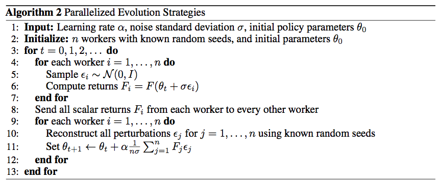
Evolution strategies and RL parallel training
Errata: The original formula in the post is wrong. I have updated it to the correct one.
$$ \begin{aligned} & \color{red}{J(\mu)=\mathbb E_{\theta\sim N(\mu,\sigma^2I)}[F(\theta)]} \\ \\ & \color{red}{\nabla_\mu J(\mu)} \\ =& \color{red}{ \nabla_\mu \int F(\theta) \,p(\theta;\mu) \,d\theta } \\ =& \color{red}{ \int F(\theta) \,\nabla_\mu p(\theta;\mu) \,d\theta } \qquad \text{\color{red}{(move gradient inside the integral)}} \\ =& \int F(\theta) \,p(\theta;\mu) \, \frac{\nabla_\mu p(\theta;\mu)} {p(\theta;\mu)} \,d\theta \\ =& \int F(\theta) \,p(\theta;\mu) \, \nabla_\mu \log p(\theta;\mu) \,d\theta \\ =& \mathbb E_{\theta\sim N(\mu,\sigma^2I)} \Big[ F(\theta) \nabla_\mu \log p(\theta;\mu) \Big] \\ =& \mathbb E_{\theta\sim N(\mu,\sigma^2I)} \Bigg[ F(\theta) \nabla_\mu \log \Bigg( \frac{1} {\sqrt{2\pi\sigma^2}} e^{-\frac{(\theta-\mu)^2}{2\sigma^2}} \Bigg) \Bigg] \\ =& \mathbb E_{\theta\sim N(\mu,\sigma^2I)} \Bigg[ F(\theta) \nabla_\mu \Bigg( -\log\sqrt{2\pi\sigma^2} -\frac{(\theta-\mu)^2}{2\sigma^2} \Bigg) \Bigg] \\ =& \mathbb E_{\theta\sim N(\mu,\sigma^2I)} \Bigg[ F(\theta) \frac{\theta-\mu}{\sigma^2} \Bigg] \end{aligned} $$Based on the reparameterization trick, we can sample $\epsilon \sim N(0, I)$ and estimate the gradient with:
$$ \nabla_\theta \mathbb{E}_{\epsilon \sim N(0, I)} F(\theta + \sigma \epsilon) = \frac{1}{\sigma} \mathbb{E}_{\epsilon \sim N(0, I)} [F(\theta + \sigma \epsilon) \epsilon] $$ES, as a black-box optimization algorithm, is another approach to RL problems (In my original writing, I used the phrase “a nice alternative”; Seita pointed me to this discussion and thus I updated my wording.). It has a couple of good characteristics (Salimans et al., 2017) keeping it fast and easy to train:
- ES does not need value function approximation;
- ES does not perform gradient back-propagation;
- ES is invariant to delayed or long-term rewards;
- ES is highly parallelizable with very little data communication.
No further explanation needed.
Known Problems
Exploration-Exploitation Dilemma
The problem of exploration vs exploitation dilemma has been discussed in my previous post. When the RL problem faces an unknown environment, this issue is especially a key to finding a good solution: without enough exploration, we cannot learn the environment well enough; without enough exploitation, we cannot complete our reward optimization task.
Different RL algorithms balance between exploration and exploitation in different ways. In MC methods, Q-learning or many on-policy algorithms, the exploration is commonly implemented by $\epsilon$-greedy; In ES, the exploration is captured by the policy parameter perturbation. Please keep this into consideration when developing a new RL algorithm.
And in auto-research and heuristic-learning paradigms, the exploration is implemented by LLMs’ creativity and randomness in generating new solutions.
Deadly Triad Issue
This post explains the deadly triad issue in more details.
Case Study: AlphaGo Zero
The game of Go has been an extremely hard problem in the field of Artificial Intelligence for decades until recent years. AlphaGo and AlphaGo Zero are two programs developed by a team at DeepMind. Both involve deep Convolutional Neural Networks (CNN) and Monte Carlo Tree Search (MCTS) and both have been approved to achieve the level of professional human Go players. Different from AlphaGo that relied on supervised learning from expert human moves, AlphaGo Zero used only reinforcement learning and self-play without human knowledge beyond the basic rules.
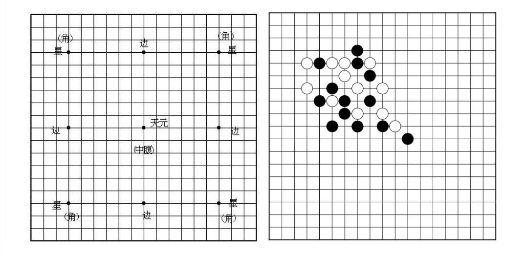
AlphaGo Zero Go board configuration
With all the knowledge of RL above, let’s take a look at how AlphaGo Zero works. The main component is a deep CNN over the game board configuration (precisely, a ResNet with batch normalization and ReLU). This network outputs two values:
$(p, v) = f_\theta(s)$
- $s$: the game board configuration, $19 \times 19 \times 17$ stacked feature planes; 17 features for each position, 8 past configurations (including current) for the current player + 8 past configurations for the opponent + 1 feature indicating the color (1=black, 0=white). We need to code the color specifically because the network is playing with itself and the colors of current player and opponents are switching between steps.
- $p$: the probability of selecting a move over $19^2 + 1$ candidates ($19^2$ positions on the board, in addition to passing).
- $v$: the winning probability given the current setting.
During self-play, MCTS further improves the action probability distribution $\pi \sim p(.)$ and then the action $a_t$ is sampled from this improved policy. The reward $z_t$ is a binary value indicating whether the current player eventually wins the game. Each move generates an episode tuple $(s_t, \pi_t, z_t)$ and it is saved into the replay memory. The details on MCTS are skipped for the sake of space in this post; please read the original paper if you are interested.
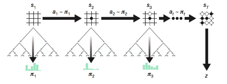
AlphaGo Zero self-play training pipeline
The network is trained with the samples in the replay memory to minimize the loss:
$$\mathcal{L} = (z - v)^2 - \pi^\top \log p + c \| \theta \|^2$$where $c$ is a hyperparameter controlling the intensity of L2 penalty to avoid overfitting.
AlphaGo Zero simplified AlphaGo by removing supervised learning and merging separated policy and value networks into one. It turns out that AlphaGo Zero achieved largely improved performance with a much shorter training time! I strongly recommend reading these two papers side by side and compare the difference, super fun.
I know this is a long read, but hopefully worth it. If you notice mistakes and errors in this post, don’t hesitate to contact me at [lilian dot wengweng at gmail dot com]. See you in the next post! :)
There is strong connection between UCT in MCTS and UCB1 in MAB.
UCT in MCTS:
$$ \mathrm{UCT}(v) = \frac{w_v}{n_v}+c\sqrt{\frac{\ln n_u}{n_v}} $$UCB1 in MAB:
$$ U_t(a) = \sqrt{\frac{2 \log t}{N_t(a)}} \text{ and } a^{UCB1}_t = \arg\max_{a \in \mathcal{A}} Q(a) + \sqrt{\frac{2 \log t}{N_t(a)}} $$| Aspect | UCT in MCTS | UCB1 in MAB |
|---|---|---|
| General Form | $\frac{w_v}{n_v} + c\sqrt{\frac{\ln n_u}{n_v}}$ | $Q(a) + \sqrt{\frac{2\ln t}{N_t(a)}}$ |
| Exploitation Term | $\frac{w_v}{n_v}$ | $Q(a)$ |
| Exploration Term | $c\sqrt{\frac{\ln n_u}{n_v}}$ | $\sqrt{\frac{2\ln t}{N_t(a)}}$ |
| Denominator (visits) | $n_v$ | $N_t(a)$ |
| Logarithmic Growth Term | $\ln n_u$ | $\ln t$ |
| Selection Rule | Choose child with max UCT | Choose arm with max UCB1 |
| Theoretical Basis | Hoeffding inequality | Hoeffding inequality |
| Goal | Balance exploration/exploitation in tree search | Balance exploration/exploitation in bandits |
| Exploration Coefficient | Tunable $c$ | Fixed $\sqrt{2}$ |
Key Formulas at a Glance
| Name | Formula |
|---|---|
| Fundamental Definitions | |
| Transition Probability | $P(s', r \vert s, a) = \mathbb{P} [S_{t+1} = s', R_{t+1} = r \vert S_t = s, A_t = a]$ |
| Discounted Return | $G_t = R_{t+1} + \gamma R_{t+2} + \dots = \sum_{k=0}^{\infty} \gamma^k R_{t+k+1}$ |
| State-Value Function | $V_{\pi}(s) = \mathbb{E}_{\pi}[G_t \vert S_t = s]$ |
| Action-Value Function | $Q_{\pi}(s, a) = \mathbb{E}_{\pi}[G_t \vert S_t = s, A_t = a]$ |
| Advantage Function | $A_{\pi}(s, a) = Q_{\pi}(s, a) - V_{\pi}(s)$ |
| Optimal Value Functions | $V_{*}(s) = \max_{\pi} V_{\pi}(s), \quad Q_{*}(s, a) = \max_{\pi} Q_{\pi}(s, a)$ |
| Bellman Equations | |
| Bellman Expectation for $V_\pi$ | $V_{\pi}(s) = \sum_{a \in \mathcal{A}} \pi(a \vert s) \big( R(s, a) + \gamma \sum_{s' \in \mathcal{S}} P_{ss'}^a V_{\pi} (s') \big)$ |
| Bellman Expectation for $Q_\pi$ | $Q_{\pi}(s, a) = R(s, a) + \gamma \sum_{s' \in \mathcal{S}} P_{ss'}^a \sum_{a' \in \mathcal{A}} \pi(a' \vert s') Q_{\pi} (s', a')$ |
| Bellman Optimality for $V_*$ | $V_{*}(s) = \max_{a \in \mathcal{A}} \big( R(s, a) + \gamma \sum_{s' \in \mathcal{S}} P_{ss'}^a V_{*}(s') \big)$ |
| Bellman Optimality for $Q_*$ | $Q_{*}(s, a) = R(s, a) + \gamma \sum_{s' \in \mathcal{S}} P_{ss'}^a \max_{a' \in \mathcal{A}} Q_{*}(s', a')$ |
| Dynamic Programming | |
| Policy Evaluation | $V_{t+1}(s) = \sum_a \pi(a \vert s) \sum_{s', r} P(s', r \vert s, a) \big(r + \gamma V_t(s')\big)$ |
| Policy Improvement | $Q_\pi(s, a) = \sum_{s', r} P(s', r \vert s, a) \big(r + \gamma V_\pi(s')\big)$ |
| Monte-Carlo Methods | |
| MC State-Value Estimate | $V(s) = \frac{\sum_{t=1}^T \mathbb{1}[S_t = s] \, G_t}{\sum_{t=1}^T \mathbb{1}[S_t = s]}$ |
| MC Action-Value Estimate | $Q(s, a) = \frac{\sum_{t=1}^T \mathbb{1}[S_t = s, A_t = a] \, G_t}{\sum_{t=1}^T \mathbb{1}[S_t = s, A_t = a]}$ |
| Temporal-Difference Learning | |
| TD(0) Value Update | $V(S_t) \leftarrow V(S_t) + \alpha \big(R_{t+1} + \gamma V(S_{t+1}) - V(S_t)\big)$ |
| SARSA (On-Policy) | $Q(S_t, A_t) \leftarrow Q(S_t, A_t) + \alpha \big(R_{t+1} + \gamma Q(S_{t+1}, A_{t+1}) - Q(S_t, A_t)\big)$ |
| Q-Learning (Off-Policy) | $Q(S_t, A_t) \leftarrow Q(S_t, A_t) + \alpha \big(R_{t+1} + \gamma \max_{a \in \mathcal{A}} Q(S_{t+1}, a) - Q(S_t, A_t)\big)$ |
| DQN Loss | $\mathcal{L}(\theta) = \mathbb{E}_{(s, a, r, s') \sim U(D)} \Big[ \big( r + \gamma \max_{a'} Q(s', a'; \theta^{-}) - Q(s, a; \theta) \big)^2 \Big]$ |
| $n$-Step Return | $G_t^{(n)} = R_{t+1} + \gamma R_{t+2} + \dots + \gamma^{n-1} R_{t+n} + \gamma^n V(S_{t+n})$ |
| $\lambda$-Return | $G_t^{\lambda} = (1-\lambda) \sum_{n=1}^{\infty} \lambda^{n-1} G_t^{(n)}$ |
| Policy Gradient Methods | |
| Policy Gradient Theorem | $\nabla \mathcal{J}(\theta) = \mathbb{E}_{\pi_\theta}[\nabla \ln \pi(a \vert s, \theta) \, Q_\pi(s, a)]$ |
| REINFORCE Update | $\theta \leftarrow \theta + \alpha \gamma^t G_t \nabla \ln \pi(A_t \vert S_t, \theta)$ |
| Actor-Critic Policy Update | $\theta \leftarrow \theta + \alpha_\theta \, Q(s, a; w) \, \nabla_\theta \ln \pi(a \vert s; \theta)$ |
| Actor-Critic TD Correction | $G_{t:t+1} = r_t + \gamma Q(s', a'; w) - Q(s, a; w)$ |
| A3C Return Estimation | $R = \begin{cases} 0 & \text{if } s_t \text{ is TERMINAL} \\ V(s_t; w') & \text{otherwise} \end{cases}$ |
| ES Gradient | $\nabla_\theta \mathbb{E}_{\epsilon \sim N(0, I)} F(\theta + \sigma \epsilon) = \frac{1}{\sigma} \mathbb{E}_{\epsilon \sim N(0, I)} [F(\theta + \sigma \epsilon) \, \epsilon]$ |
| Case Study: AlphaGo Zero | |
| AlphaGo Zero Loss | $\mathcal{L} = (z - v)^2 - \pi^\top \log p + c \| \theta \|^2$ |
Citation
@article{shichaosong2026fullyannotatedg,
  title = {Fully Annotated Guide to "A (Long) Peek into Reinforcement Learning"},
  author = {Shichao Song},
  journal = {The Kiseki Log},
  year = {2026},
  month = {May},
  url = {https://ki-seki.github.io/posts/260531-lilian-rl-overview/}
}
References
[1] Yuxi Li. Deep reinforcement learning: An overview. arXiv preprint arXiv:1701.07274. 2017.
[2] Richard S. Sutton and Andrew G. Barto. Reinforcement Learning: An Introduction; 2nd Edition. 2017.
[3] Volodymyr Mnih, et al. Asynchronous methods for deep reinforcement learning. ICML. 2016.
[4] Tim Salimans, et al. Evolution strategies as a scalable alternative to reinforcement learning. arXiv preprint arXiv:1703.03864 (2017).
[5] David Silver, et al. Mastering the game of go without human knowledge. Nature 550.7676 (2017): 354.
[6] David Silver, et al. Mastering the game of Go with deep neural networks and tree search. Nature 529.7587 (2016): 484-489.
[7] Volodymyr Mnih, et al. Human-level control through deep reinforcement learning. Nature 518.7540 (2015): 529.
[8] Ziyu Wang, et al. Dueling network architectures for deep reinforcement learning. ICML. 2016.
[9] Reinforcement Learning lectures by David Silver on YouTube.
[10] OpenAI Blog: Evolution Strategies as a Scalable Alternative to Reinforcement Learning
[11] Frank Sehnke, et al. Parameter-exploring policy gradients. Neural Networks 23.4 (2010): 551-559.
[12] Csaba Szepesvári. Algorithms for reinforcement learning. 1st Edition. Synthesis lectures on artificial intelligence and machine learning 4.1 (2010): 1-103.