Fully Annotated Guide to "The Multi-Armed Bandit Problem and Its Solutions"

This article provides a comprehensive annotated guide to Lilian Weng’s “The Multi-Armed Bandit Problem and Its Solutions”.

Exploitation vs Exploration

The exploration vs exploitation dilemma exists in many aspects of our life. Say, your favorite restaurant is right around the corner. If you go there every day, you would be confident of what you will get, but miss the chances of discovering an even better option. If you try new places all the time, very likely you are gonna have to eat unpleasant food from time to time. Similarly, online advisors try to balance between the known most attractive ads and the new ads that might be even more successful.

A real-life example of the exploration vs exploitation dilemma: where to eat? (Image source: UC Berkeley AI course [slide](http://ai.berkeley.edu/lecture_slides.html), [lecture 11](http://ai.berkeley.edu/slides/Lecture%2011%20--%20Reinforcement%20Learning%20II/SP14%20CS188%20Lecture%2011%20--%20Reinforcement%20Learning%20II.pptx).) — A real-life example of the exploration vs exploitation dilemma: where to eat? (Image source: UC Berkeley AI course slide, lecture 11.)

If we have learned all the information about the environment, we are able to find the best strategy by even just simulating brute-force, let alone many other smart approaches. The dilemma comes from the incomplete information: we need to gather enough information to make best overall decisions while keeping the risk under control. With exploitation, we take advantage of the best option we know. With exploration, we take some risk to collect information about unknown options. The best long-term strategy may involve short-term sacrifices. For example, one exploration trial could be a total failure, but it warns us of not taking that action too often in the future.

The exploration–exploitation dilemma arises because information is incomplete.
Optimal long‑term strategy requires balancing short‑term risk and long‑term gain.

What is Multi-Armed Bandit?

The multi-armed bandit problem is a classic problem that well demonstrates the exploration vs exploitation dilemma. Imagine you are in a casino facing multiple slot machines and each is configured with an unknown probability of how likely you can get a reward at one play. The question is: What is the best strategy to achieve highest long-term rewards?

In this post, we will only discuss the setting of having an infinite number of trials. The restriction on a finite number of trials introduces a new type of exploration problem. For instance, if the number of trials is smaller than the number of slot machines, we cannot even try every machine to estimate the reward probability (!) and hence we have to behave smartly w.r.t. a limited set of knowledge and resources (i.e. time).

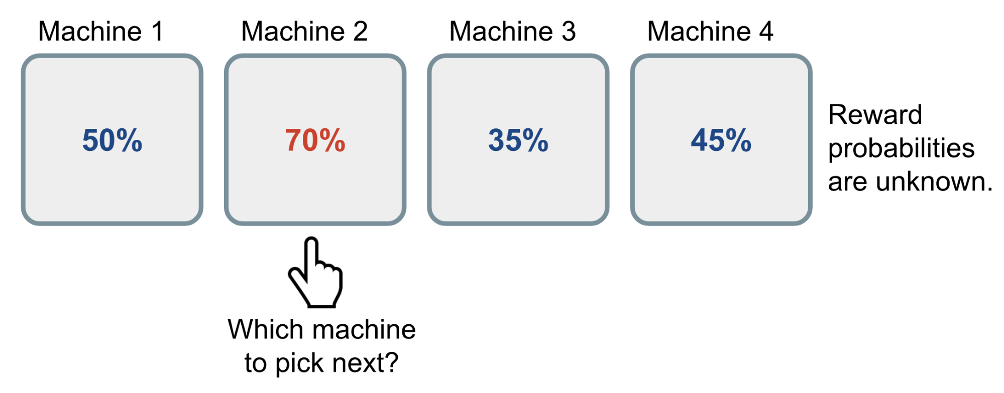
An illustration of how a Bernoulli multi-armed bandit works. The reward probabilities are **unknown** to the player.

A naive approach can be that you continue to playing with one machine for many many rounds so as to eventually estimate the “true” reward probability according to the law of large numbers. However, this is quite wasteful and surely does not guarantee the best long-term reward.

Bernoulli multi-armed bandit = Each arm has binary rewards (0 or 1)

Definition

Now let’s give it a scientific definition.

A Bernoulli multi-armed bandit can be described as a tuple of $\langle \mathcal{A}, \mathcal{R} \rangle$, where:

We have $K$ machines with reward probabilities, $\{ \theta_1, \dots, \theta_K \}$.
At each time step t, we take an action a on one slot machine and receive a reward r.
$\mathcal{A}$ is a set of actions, each referring to the interaction with one slot machine. The value of action a is the expected reward, $Q(a) = \mathbb{E} [r \vert a] = \theta$. If action $a_t$ at the time step t is on the i-th machine, then $Q(a_t) = \theta_i$.
$\mathcal{R}$ is a reward function. In the case of Bernoulli bandit, we observe a reward r in a stochastic fashion. At the time step t, $r_t = \mathcal{R}(a_t)$ may return reward 1 with a probability $Q(a_t)$ or 0 otherwise.

It is a simplified version of Markov decision process, as there is no state $\mathcal{S}$.

The goal is to maximize the cumulative reward $\sum_{t=1}^T r_t$. If we know the optimal action with the best reward, then the goal is same as to minimize the potential regret or loss by not picking the optimal action.

The optimal reward probability $\theta^{*}$ of the optimal action $a^{*}$ is:

$$ \theta^{*}=Q(a^{*})=\max_{a \in \mathcal{A}} Q(a) = \max_{1 \leq i \leq K} \theta_i $$

Our loss function is the total regret we might have by not selecting the optimal action up to the time step T:

$$ \mathcal{L}_T = \mathbb{E} \Big[ \sum_{t=1}^T \big( \theta^{*} - Q(a_t) \big) \Big] $$

Actions:

$a \in \mathcal{A} = \{1, 2, \dots, K\}$

Define an immediate value / expected reward function of a specific action:

$Q(a) = \mathbb{E} [r \vert a] = 1 * \theta_a + 0 * (1-\theta_a)$
We prefer $\mathbb{E} [r \vert a]$ rather than $Pr(r=1 \vert a)$.
If it is a Gaussian bandit, the reward can be a continuous value and the expected reward is not the same as the probability of getting a reward (r=1).

If at time step t, we take action on the i-th machine:

$Q(a_t=i) = \theta_i$

Define the reward function:

$$ r = \mathcal{R}(a) = \begin{cases} 1 & \text{with probability } \theta_a \\ 0 & \text{with probability } 1-\theta_a \end{cases} $$

Bernoulli multi-armed bandit is simplified Markov decision process because:

There is no state transition.
The reward only depends on the current action,
not the history of actions and rewards.

Our objective:

$\max \sum_{t=1}^T r_t$

The optimal strategy is to always select the optimal action $a^{*}$ with the highest reward probability $\theta^{*}$:

$$ \begin{align} \max_{a \in \mathcal{A}} Q(a) &= \max_{1 \leq i \leq K} \theta_i \\ Q(a^{*}) &= \theta^{*} \end{align} $$

In different distribution settings, the $\theta^{*}$ can be defined differently. It can be regarded as an abstract environment parameter.

Reward Distribution	$θ_i$ Meaning
Bernoulli	Win probability
Gaussian	Mean $μ_i$
Poisson	Event rate $λ_i$
Exponential	Rate parameter $1/λ_i$

Let’s finally see the Loss / Regret function:

$$ \mathcal{L}_T = \mathbb{E} \Big[ \sum_{t=1}^T \big( \theta^{*} - Q(a_t) \big) \Big] $$

It’s quite intuitive except another expectation operator $\mathbb{E}$ outside the summation.

Expectation in $Q(a)$: because the reward is stochastic
Expectation in $\mathcal{L}_T$: mainly because the action trajectory is stochastic due to the exploration/policy strategy.

There are three sources of randomness in the multi-armed bandit problem:

Source of Randomness	Impact	Included in Q(a)?	Affects Regret?
reward randomness	r is random	✔ Included in Q(a)	✔ Affects estimation
policy randomness	policy itself is random	✘	✔
estimation randomness	reward noise leads to different estimates	✘	✔

Bandit Strategies

Strategies

Based on how we do exploration, there several ways to solve the multi-armed bandit.

No exploration: the most naive approach and a bad one.
Exploration at random
Exploration smartly with preference to uncertainty

Category	Strategy Name	How It Works
No exploration	Greedy	Always pick the arm with the highest current estimated value $\hat{Q}(a)$
Random exploration	ε‑Greedy	With prob. $1-\varepsilon$ pick best arm; with prob. $\varepsilon$ pick a random arm
Smart exploration (uncertainty‑driven)	UCB (Upper Confidence Bound)	Pick arm maximizing $\hat{Q}(a) + \text{uncertainty bonus}$
Smart exploration (probabilistic)	Thompson Sampling	Sample a parameter from each arm’s posterior; pick the arm with the highest sample

ε-Greedy Algorithm

The ε-greedy algorithm takes the best action most of the time, but does random exploration occasionally. The action value is estimated according to the past experience by averaging the rewards associated with the target action a that we have observed so far (up to the current time step t):

$$ \hat{Q}_t(a) = \frac{1}{N_t(a)} \sum_{\tau=1}^t r_\tau \mathbb{1}[a_\tau = a] $$

where $\mathbb{1}$ is a binary indicator function and $N_t(a)$ is how many times the action a has been selected so far, $N_t(a) = \sum_{\tau=1}^t \mathbb{1}[a_\tau = a]$.

According to the ε-greedy algorithm, with a small probability $\epsilon$ we take a random action, but otherwise (which should be the most of the time, probability 1-$\epsilon$) we pick the best action that we have learnt so far: $\hat{a}^{*}_t = \arg\max_{a \in \mathcal{A}} \hat{Q}_t(a)$.

Check my toy implementation.

$\hat{Q}_t(a)$ is the algorithm’s estimate of the true value $Q(a)$, and it is used to guide exploitation.
$\hat{Q}_t(a)$ represents the algorithm’s belief about the value of action $a$, not the true value itself.

Upper Confidence Bounds

The Intent of UCB

Random exploration gives us an opportunity to try out options that we have not known much about. However, due to the randomness, it is possible we end up exploring a bad action which we have confirmed in the past (bad luck!). To avoid such inefficient exploration, one approach is to decrease the parameter ε in time and the other is to be optimistic about options with high uncertainty and thus to prefer actions for which we haven’t had a confident value estimation yet. Or in other words, we favor exploration of actions with a strong potential to have a optimal value.

UCB is designed to be optimistic under uncertainty:

If an arm has high estimated value → good
If an arm has high uncertainty → also good
If an arm has both → UCB will pick it even if its true value is not the best

UCB formulation

The Upper Confidence Bounds (UCB) algorithm measures this potential by an upper confidence bound of the reward value, $\hat{U}_t(a)$, so that the true value is below with bound $Q(a) \leq \hat{Q}_t(a) + \hat{U}_t(a)$ with high probability. The upper bound $\hat{U}_t(a)$ is a function of $N_t(a)$; a larger number of trials $N_t(a)$ should give us a smaller bound $\hat{U}_t(a)$.

In UCB algorithm, we always select the greediest action to maximize the upper confidence bound:

$$ a^{UCB}_t = argmax_{a \in \mathcal{A}} \hat{Q}_t(a) + \hat{U}_t(a) $$

Now, the question is how to estimate the upper confidence bound.

Term	Depends on $N_t(a)$ because…	Purpose
$\hat{Q}_t(a)$	more samples → better mean estimate	exploitation
$\hat{U}_t(a)$	more samples → less uncertainty	exploration

Why do we use an upper bound rather than a lower bound or a confidence interval?
We use an upper bound because exploration is about finding actions that might be optimal, and only the upper bound captures that potential.

Hoeffding’s Inequality

Hoeffding's Inequality

If we do not want to assign any prior knowledge on how the distribution looks like, we can get help from “Hoeffding’s Inequality” — a theorem applicable to any bounded distribution.

Let $X_1, \dots, X_t$ be i.i.d. (independent and identically distributed) random variables and they are all bounded by the interval $[0, 1]$. The sample mean is $\overline{X}_t = \frac{1}{t}\sum_{\tau=1}^t X_\tau$. Then for $u > 0$, we have:

$$ \mathbb{P} [ \mathbb{E}[X] > \overline{X}_t + u] \leq e^{-2tu^2} $$

Given one target action $a$, let us consider:

$r_t(a)$ as the random variables,
$Q(a)$ as the true mean,
$\hat{Q}_t(a)$ as the sample mean,
And $u$ as the upper confidence bound, $u = U_t(a)$

Then we have,

$$ \mathbb{P} [ Q(a) > \hat{Q}_t(a) + U_t(a)] \leq e^{-2t{U_t(a)}^2} $$

We want to pick a bound so that with high chances the true mean is blow the sample mean + the upper confidence bound. Thus $e^{-2t U_t(a)^2}$ should be a small probability. Let’s say we are ok with a tiny threshold p:

$$ e^{-2t U_t(a)^2} = p \text{ Thus, } U_t(a) = \sqrt{\frac{-\log p}{2 N_t(a)}} $$

Set $e^{-2t U_t(a)^2} = p$, then $U_t(a) = \sqrt{\frac{-\log p}{2 N_t(a)}}$
$p \downarrow \Rightarrow U_t(a) \uparrow$

$$ \begin{align} & \mathbb{P} [ Q(a) > \hat{Q}_t(a) + U_t(a)] \leq e^{-2t{U_t(a)}^2} \\ \Rightarrow\; & Q(a) > \hat{Q}_t(a) + U_t(a) \text{ holds with probability at most } e^{-2t{U_t(a)}^2} \\ \Rightarrow\; & Q(a) \leq \hat{Q}_t(a) + U_t(a) \text{ holds with probability at least } 1 - e^{-2t{U_t(a)}^2} \\ \Rightarrow\; & Q(a) \leq \hat{Q}_t(a) + \sqrt{\frac{-\log p}{2 N_t(a)}} \text{ holds with probability at least } 1-p \end{align} $$

Here, $p$ is a hyperparameter that we can adjust.

UCB1

UCB1 algorithm

One heuristic is to reduce the threshold p in time, as we want to make more confident bound estimation with more rewards observed. Set $p=t^{-4}$ we get UCB1 algorithm:

$$ U_t(a) = \sqrt{\frac{2 \log t}{N_t(a)}} \text{ and } a^{UCB1}_t = \arg\max_{a \in \mathcal{A}} Q(a) + \sqrt{\frac{2 \log t}{N_t(a)}} $$

A smaller $p$ means a more strict confidence requirement and thus a larger upper confidence bound, which encourages more exploration.
Let’s see an example. If we always choose the same action and, then $N_t(a) = t$ and $U_t(a) = \sqrt{\frac{2 \log t}{t}}$. As $t$ increases, $U_t(a)$ decreases, which means we are more confident about the estimation of that action’s value and thus we are less likely to explore it.

Bayesian UCB

About the prior

In UCB or UCB1 algorithm, we do not assume any prior on the reward distribution and therefore we have to rely on the Hoeffding’s Inequality for a very generalize estimation. If we are able to know the distribution upfront, we would be able to make better bound estimation.

We know the reward distribution is Bernoulli.
We don’t know the reward distribution’s parameter $\theta$.
Parameter $\theta$ is the prior knowledge we can use to make better estimation of the upper confidence bound.

Gaussian mean reward

For example, if we expect the mean reward of every slot machine to be Gaussian as in Fig 2, we can set the upper bound as 95% confidence interval by setting $\hat{U}_t(a)$ to be twice the standard deviation.

When the expected reward has a Gaussian distribution. $\sigma(a_i)$ is the standard deviation and $c\sigma(a_i)$ is the upper confidence bound. The constant $c$ is a adjustable hyperparameter. (Image source: [UCL RL course lecture 9's slides](http://www0.cs.ucl.ac.uk/staff/d.silver/web/Teaching_files/XX.pdf)) — When the expected reward has a Gaussian distribution. $\sigma(a_i)$ is the standard deviation and $c\sigma(a_i)$ is the upper confidence bound. The constant $c$ is a adjustable hyperparameter. (Image source: UCL RL course lecture 9’s slides)

Check my toy implementation of UCB1 and Bayesian UCB with Beta prior on θ.

$X \sim \mathcal N(\mu,\sigma^2) \Rightarrow P(X > \mu + z_\alpha \sigma) = \alpha$
$Q_t(a) \sim \mathcal N(\hat{Q}_t(a), \sigma^2(a)) \Rightarrow P(Q_t(a) > \hat{Q}_t(a) + z_\alpha \sigma(a)) = \alpha$
When $\alpha=0.05$, we have $z_\alpha \approx 1.645$ and thus the upper confidence bound is $\hat{Q}_t(a) + 1.645 \sigma(a)$, which means that the true value is below the upper confidence bound with a probability at least $1-5\%=95\%$.
Note: The commonly used $2\sigma$ bound is actually a two-sided confidence interval with $\alpha/2 = 0.025$. The author may make a mistake.

Thompson Sampling

Thompson sampling has a simple idea but it works great for solving the multi-armed bandit problem.

Oops, I guess not this Thompson? (Credit goes to [Ben Taborsky](https://www.linkedin.com/in/benjamin-taborsky); he has a full theorem of how Thompson invented while pondering over who to pass the ball. Yes I stole his joke.) — Oops, I guess not this Thompson? (Credit goes to Ben Taborsky; he has a full theorem of how Thompson invented while pondering over who to pass the ball. Yes I stole his joke.)

At each time step, we want to select action a according to the probability that a is optimal:

$$ \begin{aligned} \pi(a \; \vert \; h_t) &= \mathbb{P} [ Q(a) > Q(a'), \forall a' \neq a \; \vert \; h_t] \\ &= \mathbb{E}_{\mathcal{R} \vert h_t} [ \mathbb{1}(a = \arg\max_{a \in \mathcal{A}} Q(a)) ] \end{aligned} $$

where $\pi(a ; \vert ; h_t)$ is the probability of taking action a given the history $h_t$.

For the Bernoulli bandit, it is natural to assume that $Q(a)$ follows a Beta distribution, as $Q(a)$ is essentially the success probability θ in Bernoulli distribution. The value of $\text{Beta}(\alpha, \beta)$ is within the interval $[0, 1]$; α and β correspond to the counts when we succeeded or failed to get a reward respectively.

First, let us initialize the Beta parameters α and β based on some prior knowledge or belief for every action. For example,

α = 1 and β = 1; we expect the reward probability to be 50% but we are not very confident.
α = 1000 and β = 9000; we strongly believe that the reward probability is 10%.

At each time t, we sample an expected reward, $\tilde{Q}(a)$, from the prior distribution $\text{Beta}(\alpha_i, \beta_i)$ for every action. The best action is selected among samples: $a^{TS}_t = \arg\max_{a \in \mathcal{A}} \tilde{Q}(a)$. After the true reward is observed, we can update the Beta distribution accordingly, which is essentially doing Bayesian inference to compute the posterior with the known prior and the likelihood of getting the sampled data.

$$ \begin{aligned} \alpha_i & \leftarrow \alpha_i + r_t \mathbb{1}[a^{TS}_t = a_i] \\ \beta_i & \leftarrow \beta_i + (1-r_t) \mathbb{1}[a^{TS}_t = a_i] \end{aligned} $$

Thompson sampling implements the idea of probability matching. Because its reward estimations $\tilde{Q}$ are sampled from posterior distributions, each of these probabilities is equivalent to the probability that the corresponding action is optimal, conditioned on observed history.

However, for many practical and complex problems, it can be computationally intractable to estimate the posterior distributions with observed true rewards using Bayesian inference. Thompson sampling still can work out if we are able to approximate the posterior distributions using methods like Gibbs sampling, Laplace approximate, and the bootstraps. This tutorial presents a comprehensive review; strongly recommend it if you want to learn more about Thompson sampling.

The formula defines an ideal probability, not the algorithm. It says “$\pi(a \; \vert \; h_t)$ is the probability that action a is truly the best,” but it does not describe how to compute that probability.
The probability is taken over the posterior distributions of Q(a). Q(a) is treated as a random variable with uncertainty, so the formula is about comparing random draws of Q(a), not fixed values.
The expectation form is just a mathematical rewrite. $\mathbb{E}_{\mathcal{R} \vert h_t} [ \mathbb{1}(a = \arg\max_{a \in \mathcal{A}} Q(a)) ]$ means “the chance that a random draw of all Q’s makes action a the largest,” but still does not specify how to obtain those draws. $\mathcal{R}$ is the randomness coming from the posterior distributions of the action values $Q(a)$.
Thompson Sampling uses sampling as the practical way to realize this probability. By drawing one sample from each posterior and taking the argmax, the algorithm ensures that the frequency of selecting action a matches exactly the probability defined by the formula.

Thompson Sampling is to greedy selection what a VAE is to a standard autoencoder:

both replace a single deterministic estimate with sampling from a learned distribution.
This stochasticity lets them explore more possibilities and avoid getting trapped in narrow, overconfident solutions.

Below is a good learning resource for understanding the Beta distribution.

Case Study

I implemented the above algorithms in lilianweng/multi-armed-bandit. A BernoulliBandit object can be constructed with a list of random or predefined reward probabilities. The bandit algorithms are implemented as subclasses of Solver, taking a Bandit object as the target problem. The cumulative regrets are tracked in time.

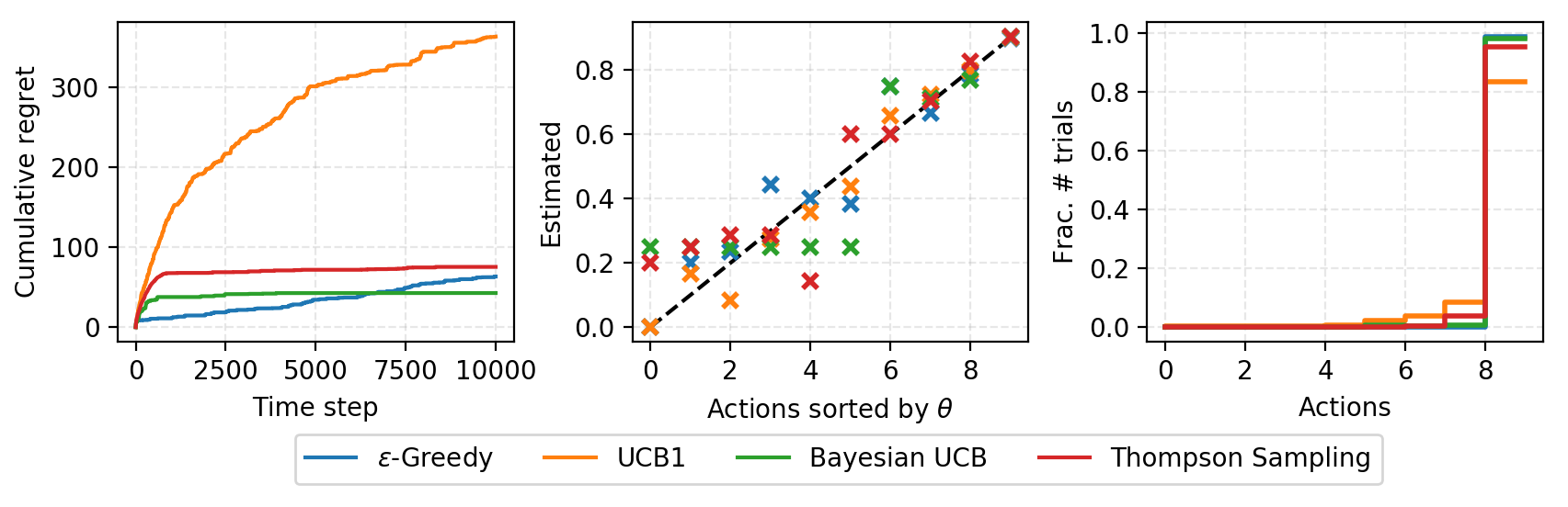
The result of a small experiment on solving a Bernoulli bandit with K = 10 slot machines with reward probabilities, . Each solver runs 10000 steps.

(Left) The plot of time step vs the cumulative regrets. (Middle) The plot of true reward probability vs estimated probability. (Right) The fraction of each action is picked during the 10000-step run.

Summary

We need exploration because information is valuable. In terms of the exploration strategies, we can do no exploration at all, focusing on the short-term returns. Or we occasionally explore at random. Or even further, we explore and we are picky about which options to explore — actions with higher uncertainty are favored because they can provide higher information gain.

Citation

@article{shichaosong2026fullyannotatedg,
  title = {Fully Annotated Guide to "The Multi-Armed Bandit Problem and Its Solutions"},
  author = {Shichao Song},
  journal = {The Kiseki Log},
  year = {2026},
  month = {April},
  url = {https://ki-seki.github.io/posts/260430-multi-armed-bandit/}
}

References

[1] CS229 Supplemental Lecture notes: Hoeffding’s inequality.

[2] RL Course by David Silver - Lecture 9: Exploration and Exploitation

[3] Olivier Chapelle and Lihong Li. “An empirical evaluation of thompson sampling.” NIPS. 2011.

[4] Russo, Daniel, et al. “A Tutorial on Thompson Sampling.” arXiv:1707.02038 (2017).

Exploitation vs Exploration#

What is Multi-Armed Bandit?#

Definition#

Bandit Strategies#

ε-Greedy Algorithm#

Upper Confidence Bounds#

Hoeffding’s Inequality#

UCB1#

Bayesian UCB#

Thompson Sampling#

Case Study#

Summary#

Citation#

References#

Exploitation vs Exploration

What is Multi-Armed Bandit?

Definition

Bandit Strategies

ε-Greedy Algorithm

Upper Confidence Bounds

Hoeffding’s Inequality

UCB1

Bayesian UCB

Thompson Sampling

Case Study

Summary

Citation

References